Session 02/Excel 2: Lookups and tables

Complete special IF functions (if necessary)

flowchart

  subgraph AFTER_BREAK["<b>After break: Excel tables</b>"]
    direction TB
    B1["<b>Create Excel Tables</b> (15 min)"]
    B2["<b>Sort, filter, design, and style</b> (15 min)"]
    B3["<b>Dynamic tables, charts, and row operations</b> (20 min)"]
    B4["<b>Total Row and SUBTOTAL</b> (15 min)"]
    B5["<b>Structured references</b> (10 min)"]
    B6["<b>💻 Exercise: Excel Tables</b> (15 min) · Sales_table"]
    B1 --> B2 --> B3 --> B4 --> B5 --> B6
  end

  subgraph BEFORE_BREAK["<b>Before break: Lookups</b>"]
    direction TB
    A1["<b>Review homework</b> (15 min) · Session 1 solutions"]
    A2["<b>VLOOKUP and HLOOKUP</b> (40 min) · 💻 Exercise: Bar sales"]
    A3["<b>XLOOKUP vs. VLOOKUP</b> (30 min) · 💻 Exercise: Client lookup"]
    A4["<b>Introduce lookup homework</b> (5 min) · Christmas gift, Course grading"]
    A1 --> A2 --> A3 --> A4
  end

Note: PR: Session 2 typically ends at 46. GW: try to cover everything until p.52

Survey follow-up

Follow-up on questions/feedback from last session’s survey.

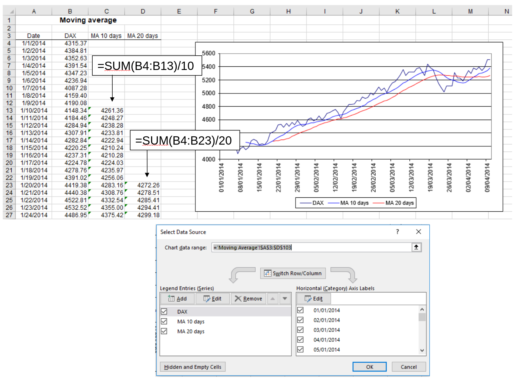
Homework review: DAX moving averages

Tip

Solve the homework in the “empty” sheet of the group’s Excel file.

Homework solution ../materials/session_01/exercises_with_solutions.xlsx – Sheet: Moving Average

Start by briefly explaining the task (again):

Discuss the spreadsheet structure before discussing individual formulas.
Check the starting periods for the 10-period and 20-period averages (sufficient historical data accumulation is needed / we cannot start in the first row with formulas1)
Emphasize that a longer moving average is smoother and reacts more slowly.

Homework review: Installment loan

Homework solution ../materials/session_01/exercises_with_solutions.xlsx – Sheet: Installment

Explain the payment schema introduced in the previous session.

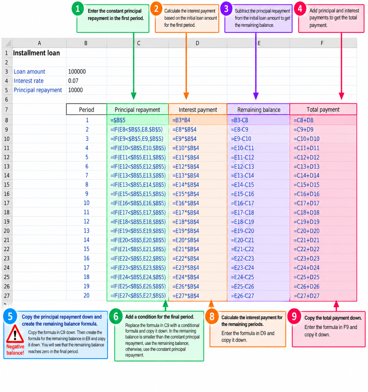
Validation:

Show how changes in Loan amount, Interest rate and Redemption are automatically reflected in the payments. This could be used in a What-if or scenario analysis.

Typical error: If the principal or interest repayments point to the same column (instead of the previous period), a “circular reference” error will be raised.

Homework review: Annuity loan

Homework solution ../materials/session_01/exercises_with_solutions.xlsx – Sheet: Annuity

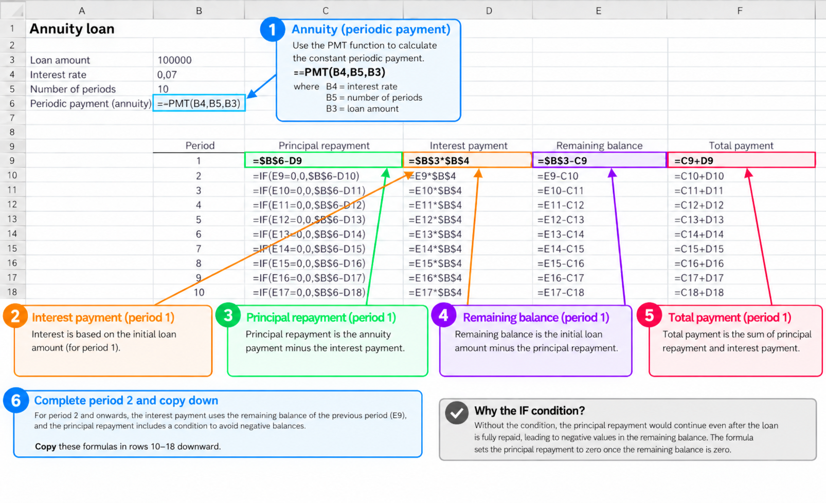
Validation:

Show that the annuity and payments per period change when modifying the numbers of periods.

Add charts for the payments of installment loans and annuity loans. Briefly contrast the declining payments of a fixed-principal loan with the constant payments of an annuity loan.

Note: Other solutions are possible (including a =MIN(...)for the principal repayment).

Lecture

Slides

If Special IF functions were not covered in the previous session: complete slide 28.

Slides 30–31 — `VLOOKUP`

Start with the practical example:

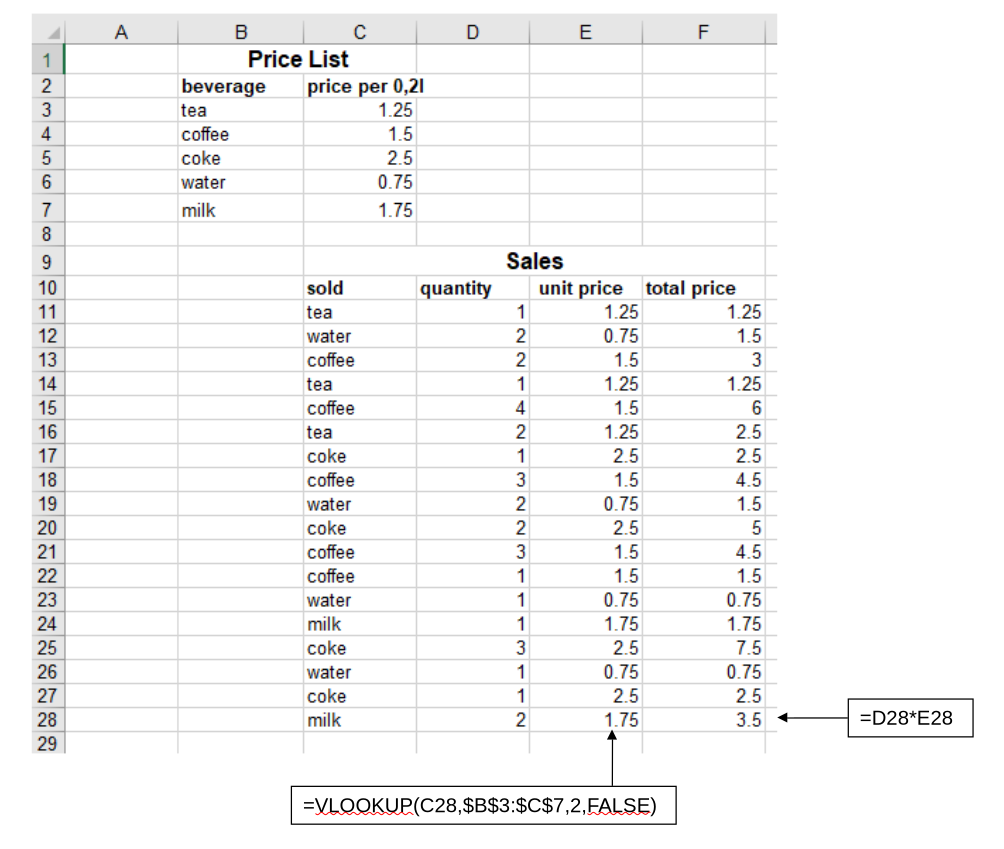
In-class demo ../materials/session_01/exercises.xlsx – Sheet: Bar_Sales

Scroll down (hide the price list initially) to start with a simple approach: filling in raw data
Highlight that this is not how a restaurant works. It does not make sense that every sale can have a different price for the same product (the unit price should not be in the sales table).
Common problem: some data (unit prices) should not be entered in the sales table, but taken from the menu.
Scroll up to the price list and explain.
Instead of copying data from the price list, we would like to use a formula: VLOOKUP

Whiteboard:

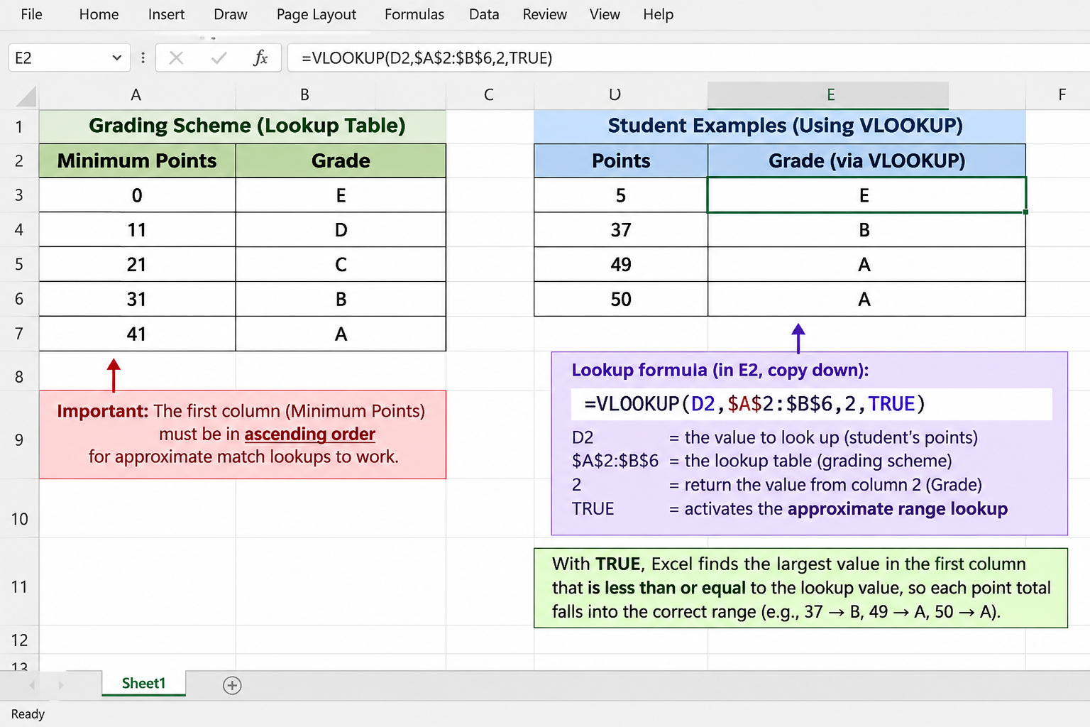
=VLOOKUP(lookup_value, table_array, column_index_num, range_lookup)

Explain parameters (range_lookup: FALSE for exact match; for TRUE/approximate matches, the first column must be sorted in ascending order)
Write VLOOKUP formula
Ask about the need for absolute and relative references
Calculate total price
Copy formulas down

Continue on the slides (the general VLOOKUP formula).

Explain the lookup process step by step:

Search for the lookup value in the first column of the selected range.
Identify the corresponding row.
Return the value from the specified column of that row.

Key points:

The lookup column must be the leftmost column in the selected range.
The return column is identified by a number rather than by its name.
Use FALSE for an exact match.
Approximate matching with TRUE should only be used deliberately and normally requires sorted lookup data.
Lock the lookup range before copying a formula down.

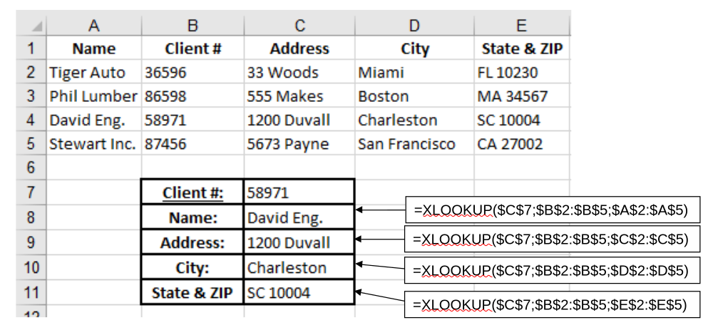
Slide 34 — Client lookup

In-class exercise ../materials/session_01/exercises.xlsx – Sheet: Clients

We want to change the client number (type in different values) and then the following fields should update automatically (based on the list above).

Teaching sequence:

Identify the client-number column as the lookup array.
Create VLOOKUP formulas for the following fields (highlight in yellow):
- Not Name
- Address
- City
- State and ZIP code
Show that the name can be returned even though it is located to the left of the client number.
Change the client number to test all formulas.

Approximate range lookups

`VLOOKUP` and `HLOOKUP`

HLOOKUP follows the same principle but searches in the first row instead of the first column.
Illustration: In the Bar_Sales table, copy the price list and paste it in transposed mode. Replace VLOOKUPs with HLOOKUPs.

Slide 33 — `XLOOKUP`

Limitation of VLOOKUP

Funny illustration: With VLOOKUP, Microsoft built a formula that can only look to the right. This is why they needed to build the XLOOKUP 😊
“VLOOKUP can only return values from columns to the right of the lookup column”
In the Client example, we cannot retrieve the Names because they are left of ClientID
This motivates the introduction of XLOOKUP.

General form:

=XLOOKUP(lookup_value, lookup_array, return_array)

Contrast it with VLOOKUP:

`VLOOKUP`	`XLOOKUP`
Searches only in the first column of the selected range	Lookup and return arrays are selected separately
Cannot directly return a value to the left	Can return values from either side
Uses a numerical column index	Uses an explicit return range
Approximate match is the default	Exact match is the default
May break when columns are inserted or reordered	More robust to structural changes

Revisiting Client exercise

Ask Students to fill in the formula to retrieve Names in the Clients sheet.
Next, the following lookups could be replaced with XLOOKUPs (in a copy of the sheet).

Slide 35 — Christmas gift (Homework)

Homework ../materials/session_01/exercises.xlsx – Sheet: Gift

Students should retrieve two values based on customer status:

Christmas gift
Packaging

Formulas are needed for the ChristmasGift and Packaging columns (each retrieving the data from a different table).

Encourage students to build both a VLOOKUPand XLOOKUP solution (demonstrate how to copy the spreadsheet).

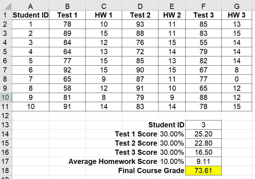
Slide 36 — Course grading (Homework)

Homework ../materials/session_01/exercises.xlsx – Sheet: Grading

This one is similar to the client lookup. We want to enter different StudentIDs and then the lookup functions should retrieve the different test scores and do the calculations of final grades.

Error on the slides

On the slides, the contribution of homework should be 9.11 and the overall grade 73.61 (as in the screenshot above).

Show the correct version to students: PDF in Canvas (images/excel_grading_assignment.png)

Break — 10 minutes

Slides 38–39 — Introduction to Excel Tables

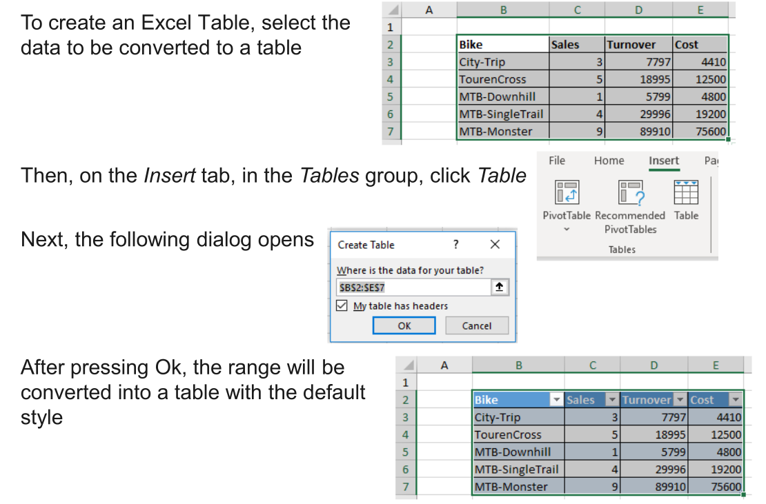
In-class demo ../materials/session_01/exercises.xlsx – Sheet: Bike_sales

Create the table together with the students. Copy and show how the range of cells behaves differently compared to the excel table

Teaching sequence:

Start with the ordinary range in the Bike_sales sheet
Illustrate shortcoming: Add Sum(range....), and then add a row in the table to show that the new data is not considered
Select the complete data range.
Insert an Excel Table (through ribbon or click into the table and use ctrl+t).
Confirm that the range contains headers.
Rename the table from its default name to Bikesales.

Explain the main differences between an ordinary range and an Excel Table:

Named object
Automatic headers
Dynamic expansion (using tab in the last line) - with updating of formulas (show and updated Sum(Bikesales[price]) example).
Integrated filtering and sorting
Structured references
Automatically propagated formulas (when adding a column, and entering a formula, it gets copied to the following cells)

Important

A table name identifies the table independently of its position in the worksheet.

Slide 40 — Sorting and filtering

Demonstrate:

Sorting by bike name.
Sorting numerical columns.
Filtering the table to selected bike models.
Removing the filter and restoring all rows.

Emphasize that filtering hides records but does not delete them. This distinction becomes important for SUBTOTAL.

Slides 41–42 — Table design and styles

With a cell inside the table selected, open Table Design.

Demonstrate:

Renaming the table.
Header Row.
Total Row.
Banded Rows and Banded Columns.
First Column and Last Column.
Filter Button.
Selecting a predefined table style.

Avoid spending too much time on visual formatting. The main purpose is to show that the table is a managed Excel object.

Slide 43 — Dynamic data entry and charts

Demonstrate that:

A new row entered immediately below the table becomes part of the table (shortcut: tab).
Table formatting is applied automatically.
Formulas in calculated columns are copied automatically.
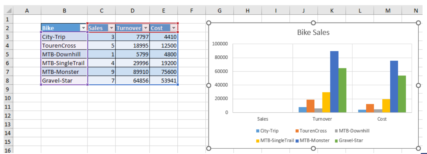
A chart based on the table expands when new data are added.

Add the Gravel-Star row and observe whether the chart changes.

Slide 44 — Inserting and deleting rows and columns

Distinguish between:

Inserting a worksheet row.
Inserting a table row.
Deleting worksheet cells.
Deleting a complete table row or column.

Students should understand that table operations affect the table structure, whereas worksheet operations may shift unrelated cells.

Slide 45 — Calculating totals

Activate Table Design → Total Row.

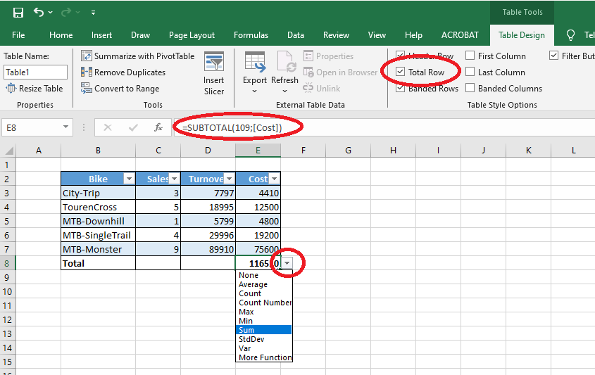
Demonstrate how the drop-down menu can be used to calculate:

Sum
Average
Count
Maximum
Minimum

Show the generated formula:

=SUBTOTAL(109,[Cost])

Key observation:

Excel does not use a normal SUM formula.
It generates a SUBTOTAL formula that responds to filtering.

Slide 46 — `SUBTOTAL` function numbers

Note

Need to select/click function or insert the Function numbers! But do not memorize them - a mapping table will be provided in the exam.

General form:

=SUBTOTAL(function_num,reference)

The first argument encodes the aggregation function:

Function	Includes manually hidden rows	Excludes manually hidden rows
`AVERAGE`	1	101
`COUNT`	2	102
…	…	…

Important: Difference between numbers 1-11 and 101-111 is manually hidden rows NOT filtered-out rows (they are always excluded from SUBTOTALs).

Function numbers	Manually hidden rows	Filtered-out rows
1–11	Included	Excluded
101–111	Excluded	Excluded

Important distinction

Filtered-out rows are excluded by SUBTOTAL.

For manually hidden rows:

Function numbers 1–11 include them.
Function numbers 101–111 exclude them.

Demonstrate the difference by:

Calculating a total.
Filtering the table.
Observing the recalculated total.
Manually hiding a row.
Comparing function numbers 9 and 109.

Slides 47–50 — Structured references

Note: This part is slightly more challenging. It will help you in the Python/Pandas sessions.

Principles:

Accessing data through variables
Selecting specific columns

In Python/Pandas, this will be the same. There are no cells with row and column numbers. They are replaced by named variables.

Note: structured references work regardless of where the table is located (name references).

Basic structured references

Contrast:

=SUM(E3:E7)

with:

=SUM(Bikesales[Cost])

Explain that the structured reference:

Uses table and column names.
Is easier to interpret.
Expands automatically.
Is independent of the table’s location on the worksheet.

Components

Work through examples of structured references and explain them on the whiteboard:

Formula example	Explanation	General syntax
`Bikesales[Cost]`	Refers to the `Cost` column	`TableName[ColumnName]`
`Bikesales[[#Totals],[Turnover]]`	Refers to the `Turnover` cell in the totals row	`TableName[[#Item],[ColumnName]]`
`Bikesales[[#Totals],[Turnover]:[Cost]]`	Refers to the totals-row cells from `Turnover` to `Cost`	`TableName[[#Item],[FirstColumn]:[LastColumn]]`

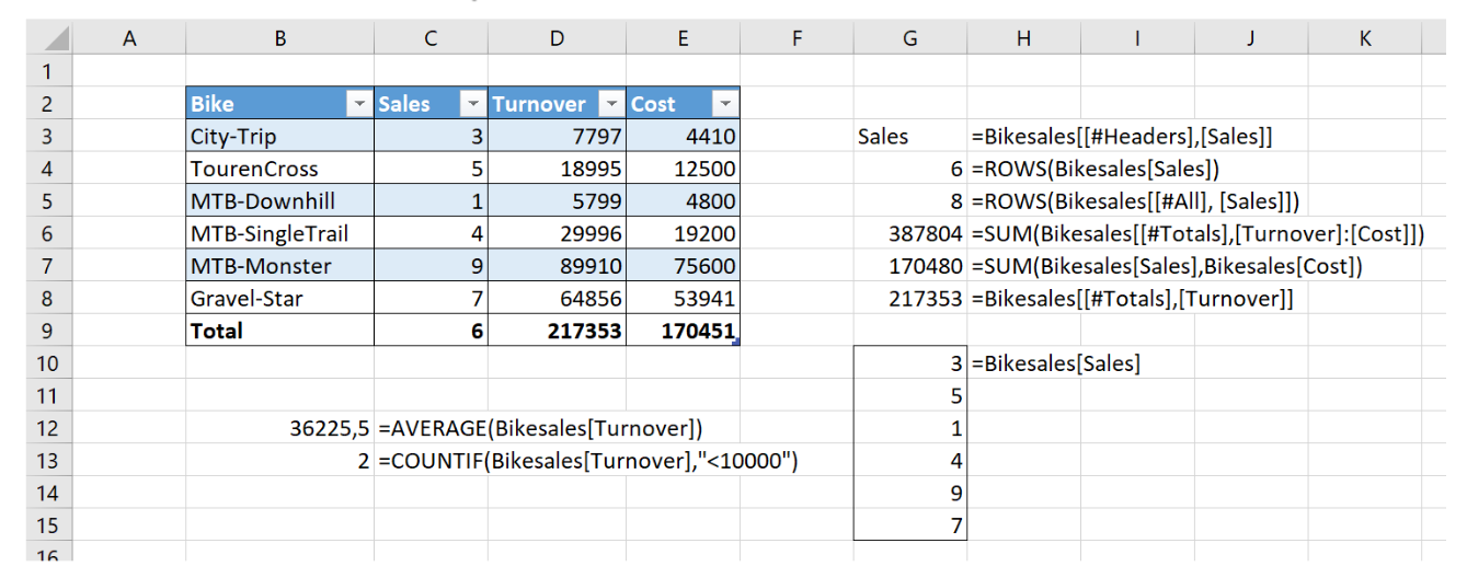
Note: in =ROWS(Bikesales[[#All],[Sales]]), the [#All] also counts header and totals as rows.

Current-row references

Working with data tables raises the question: how can we use data within the table to calculate something?

Extend the example with current row formulas (note: automated formula copying in Excel Tables!):

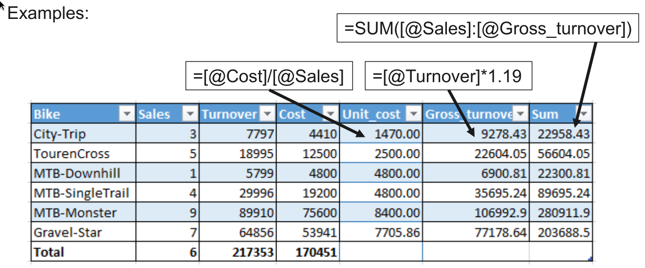
Inside the table, @ refers to the current row:

=[@Turnover]-[@Cost]
=[@Cost]/[@Sales]
=[@Turnover]*1.19

After entering the formula once, Excel should copy it to the complete calculated column.

Slides 51–52 — Excel Tables exercise

In-class exercise/Homework../materials/session_01/exercises.xlsx – Sheet: Sales_table

This extended exercise can be completed in class, assigned as homework, or continued in Session 3.

Open exercises.xlsx, sheet Sales_table, and convert the data into an Excel Table (insert > table, or ctrl+t).
Name the table Sales.
Sort the table by region (alt+down).
Filter the table to show only 2020 (alt+down + up …).
Restore all years.
Delete the records for Brazil.

Search, select values, right click, delete rows (do not press delete, which simply deletes values but not rows/records)
Enable the Total Row and calculate (use drop-down at the end of the table):
- Quantity: sum
- Cost: sum
- Turnover: average
- Year: maximum

Outside the table: Count the number of records:

=ROWS(Sales)

# Unneccesary column in the "official solution":
=ROWS(Sales[Product])

Add the column Profit:
```
=[@Turnover]-[@Cost]
```
Add the column TOpU for turnover per unit:

Before solving this task: do a plausiblity check of the numbers. Conclude that Turnover, Cost, and Profit are likely given in 1000s.
```
=[@Turnover]*1000/[@Quantity]
```
Format: reduce decimals
Add the column QShare and format it as a percentage:
```
=[@Quantity]/SUM([Quantity])
```
Format: increase decimals
In the Total Row, calculate (use drop-down at the end of the table):
- Sum of Profit
- Average of TOpU
- Sum of QShare
Outside the table: Recalculate total profit:
```
=SUM(Sales[Profit])
```
Validation check: Should be the same as the corresponding total row column.

Outside the table: Calculate total turnover in two ways:

=SUM(Sales[Turnover])

=Sales[[#Totals],[Profit]]+Sales[[#Totals],[Cost]]

Outside the table: Add all values from Year to QShare in the Total Row:

Note: As stated in the task, this makes no sense! Just for practice.
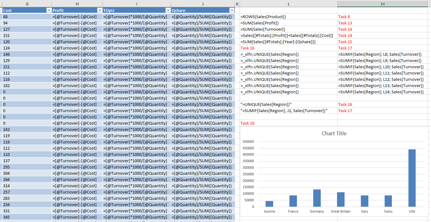
```
=SUM(Sales[[#Totals],[Year]:[QShare]])
```
Outside the table: Extract the unique regions in cell L8:
```
=UNIQUE(Sales[Region])
```
Note: The function automatically fills out the following cells.
Outside the table: Calculate turnover by region in cell M8 and fill the formula down:
```
=SUMIF(Sales[Region], L8, Sales[Turnover])
```
Outside the table: Create a chart showing total turnover by region.

Solution:

Summary and announcements

Homework:

Christmas gift
Course grading
Complete the Sales Table exercise if it was not finished in class.

Next session:

Finish structured references and the table exercise, if necessary.
Introduce PivotTables.

Notes for improvement

Take notes on timing, common errors, unclear instructions, and suitable stopping points on a separate paper and add them to feedback.qmd after the session.

Homework review: DAX moving averages

Homework review: Installment loan

Homework review: Annuity loan

Lecture

Slides 30–31 — VLOOKUP

Slide 34 — Client lookup

Approximate range lookups

VLOOKUP and HLOOKUP

Slide 33 — XLOOKUP

Revisiting Client exercise

Slide 35 — Christmas gift (Homework)

Slide 36 — Course grading (Homework)

Slides 38–39 — Introduction to Excel Tables

Slide 40 — Sorting and filtering

Slides 41–42 — Table design and styles

Slide 43 — Dynamic data entry and charts

Slide 44 — Inserting and deleting rows and columns

Slide 45 — Calculating totals

Slide 46 — SUBTOTAL function numbers

Slides 47–50 — Structured references

Basic structured references

Components

Current-row references

Slides 51–52 — Excel Tables exercise

Summary and announcements

Slides 30–31 — `VLOOKUP`

`VLOOKUP` and `HLOOKUP`

Slide 33 — `XLOOKUP`

Slide 46 — `SUBTOTAL` function numbers