Notes S-06/Python 3: Statistics, charts, and grouping

ggf. Varianz/Mittelwert erkären

Plots: nur LIne/Bar in der Klausur (siehe Dokument: relevant topics for the exam)

Note: ML/prediction is not relevant for the exam.

Focus on descriptive statistics, basic charts, filtering, and grouping; distinguish exam-relevant content from enrichment.

Slide 37 — Summing DataFrame values

The latter two expressions calculate the same sums using label-based and position-based selection.

data.sum()
exped.loc[:, ['QUANTITY', 'REVENUE']].sum()
exped.iloc[:, 5:7].sum()

Slide 39 — Mean, standard deviation, and correlation

exped.loc[:, ['QUANTITY', 'REVENUE']].mean()
exped['REVENUE'].std()
exped.loc[:, ['QUANTITY', 'REVENUE']].corr()

Slide 40 — Statistical summaries

describe() is type-aware, so its summary depends on whether the selected data are numerical or categorical.

exped.describe()
exped['REVENUE'].describe()
exped['WHERE'].describe()

Slide 41 — Unique values and frequencies

exped['WHERE'].unique()
exped['WHERE'].value_counts()

Slide 42 — Descriptive statistics

In-class exercise ../materials/data/countries.csv

In-class exercise ../materials/session_06/countries3.py

import pandas as pd

countries = pd.read_csv('countries.csv')

countries['Area'].sum()
countries['GDP'].mean()
countries['GDP'].var()

countries.loc[:, ['Population', 'Area', 'GDP']].mean()
countries.loc[[2, 10, 11, 13], ['Population', 'Area', 'GDP']].mean()

countries['Area'].min()

countries.loc[:, ['Population', 'Area', 'GDP']].corr()

countries.describe()    # or: countries[['Population', 'Area', 'GDP']].describe()

countries.loc[:, ['Country', 'Continent']].describe()

len(countries['Continent'].unique())
countries['Continent'].value_counts()

Explain variance and the mean if students need a refresher.

Slide 43 — Creating a basic chart

With no explicit column selection, plot() includes all numerical columns by default.

import pandas as pd

temps = pd.read_csv('temperatures.csv')
temps.head()
temps.plot()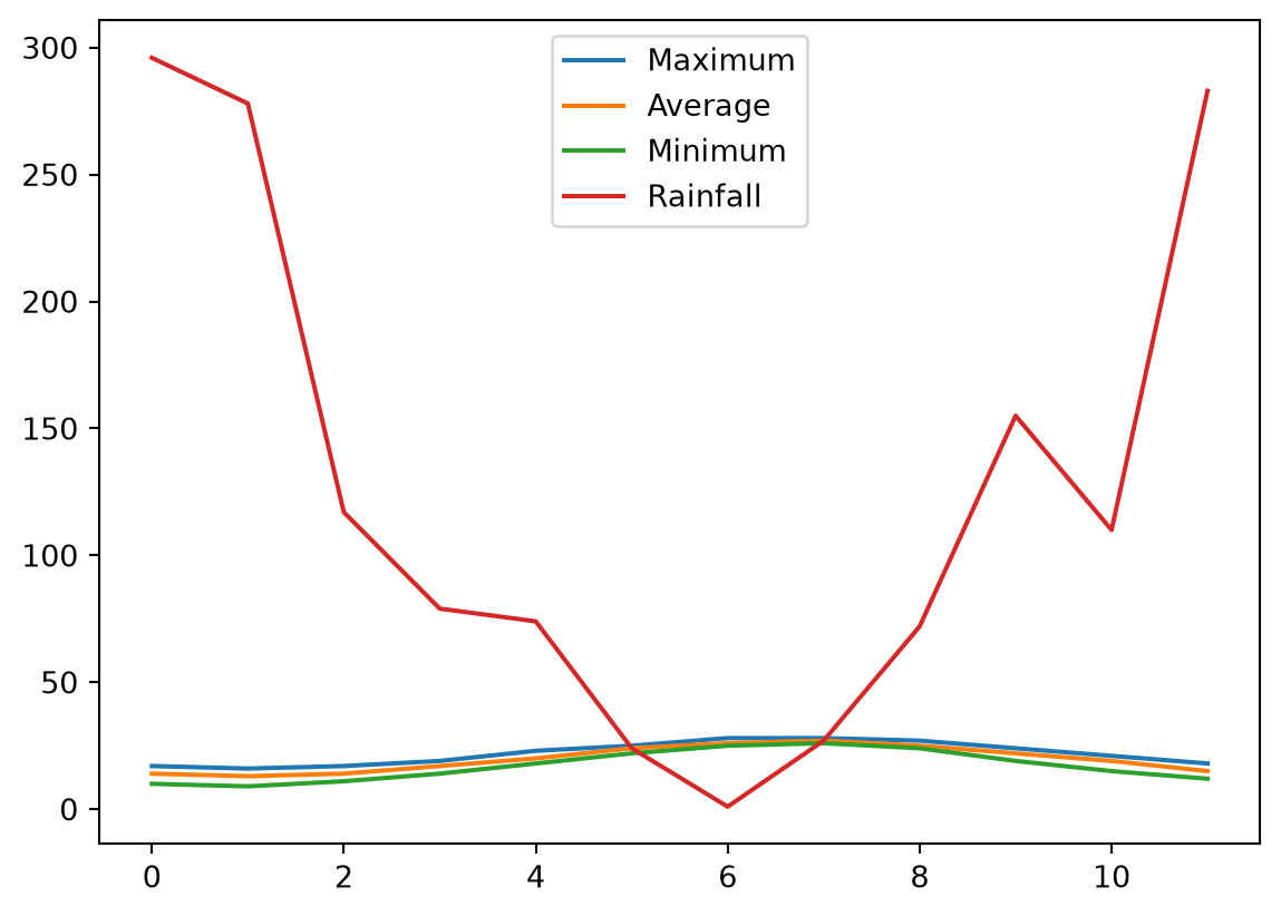

Slide 44 — Selecting variables for a chart

temps.iloc[:, 1:4].plot()
temps.plot(
    x='Month',
    y=['Maximum', 'Average', 'Minimum'],
)

Slide 45 — Formatting the x-axis

temps.plot(
    x='Month',
    y=['Maximum', 'Average', 'Minimum'],
    xticks=range(len(temps['Month'])),
    rot=75,
)

Slide 47 — Creating a bar chart

df = exped['WHERE'].value_counts()
print(df)
df.dtypes
df.plot(kind='bar')

Slide 48 — Creating pie charts

df.plot(kind='pie', y='WHERE')
df.plot(kind='pie', subplots=True)
df.plot(kind='pie', subplots=True, legend=True)

Slide 49 — Basic visualizations

In-class exercise ../materials/data/countries.csv

In-class exercise ../materials/session_06/countries4.py

import pandas as pd

countries = pd.read_csv('countries.csv')

countries.plot(x='Country', y=['Population', 'Area', 'GDP'],
               xticks=range(len(countries['Country'])), rot=75)

df = countries['Continent'].value_counts()
df.plot(kind='bar')
df.plot(kind='pie')

countries.plot(kind='density', y='GDP')
countries.plot(kind='box', y='GDP')

Exam relevance

Only line and bar plots are relevant to the exam; see the document listing exam-relevant topics.

☕ Break — 10 minutes

Slide 50 — Creating a Boolean condition

The comparison produces a Boolean Series with one value per row.

exped.WHERE == 'London'

Slide 51 — Selecting rows based on a condition

exped.loc[exped.WHERE == 'London']

Slide 52 — Combining conditions

Use & for “and” and | for “or”. Each individual pandas condition needs parentheses when conditions are combined.

exped.loc[
    (exped.WHERE == 'London')
    & (exped.REVENUE >= 2500)
]

exped.loc[
    (exped.QUANTITY >= 5)
    | (exped.REVENUE >= 2500)
]

Slide 53 — Conditional filtering

In-class exercise ../materials/data/countries.csv

In-class exercise ../materials/session_06/countries5.py

import pandas as pd

countries = pd.read_csv('countries.csv')

countries.loc[countries.Area > 8000]

countries.loc[countries.Area > 8000, 'GDP'].mean()
countries.loc[countries.Area < 800, 'GDP'].mean()

countries.loc[(countries.Area > 8000) & (countries.Population < 400)]
countries.loc[(countries.Area > 8000) & (countries.Population < 400), ['Country', 'GDP']]

df = countries.loc[(countries.Area > 8000) & (countries.Population < 400), ['Country', 'GDP']]
df.plot(x='Country', kind='bar', rot=0)

df = countries.loc[countries.Population < 100, 'Continent'].value_counts()
df.plot(kind='pie', y='Continent')

df = countries.loc[countries.Continent == 'Europe', 'GDP']
df.plot(kind='density')

Connect filtering conditions to the resulting summaries and visualizations.

Slide 54 — Grouping by one column

exped.groupby('HOW')['HOW'].count()
exped.groupby('HOW')['REVENUE'].mean()

Slide 55 — Grouping by multiple columns

a = exped.groupby(['HOW', 'WHERE'])['REVENUE'].mean()
a

Slide 56 — Grouping and aggregation

In-class exercise ../materials/data/countries.csv

In-class exercise ../materials/session_06/countries6.py

import pandas as pd

countries = pd.read_csv('countries.csv')

countries.groupby('Continent')['Continent'].count()
countries.groupby('Continent')['GDP'].mean()

countries['GDP_by_Pop'] = countries['GDP']/countries['Population']
countries.groupby('Continent')['GDP_by_Pop'].mean()

In-class exercise ../materials/data/insurance.xlsx

In-class exercise ../materials/session_06/insurance1.py

import pandas as pd

insurance = pd.read_excel('insurance.xlsx')

insurance.groupby('State')['InsuredValue'].mean()
pd.options.display.float_format = '{:.2f}'.format
insurance.groupby('State')['InsuredValue'].mean()
insurance.groupby('State')['InsuredValue'].count()
insurance.loc[insurance['Flood'] == 'Y'].groupby('State')['InsuredValue'].count()
insurance.loc[(insurance['Flood'] == 'Y') | (insurance['Earthquake'] == 'Y')].groupby('State')['InsuredValue'].count()

Demonstrate grouping with both the country and insurance datasets.

Exam relevance

Machine learning and prediction are not relevant to the exam.

Summary and announcements

TODO

Notes for improvement

Take notes on improvements and common questions during the session and add them to feedback.qmd afterwards.