Session 05/Python 2: Data access and manipulation

Preparation

Upoad the customers.xlsx
Make customers.xlsx available on presentation laptop (always use the same/unchanged file because students will try to reproduce the results)
During the code illustrations: instead of removing/replacing examples, move them to comments

flowchart

  subgraph RIGHT["<b>Modify and sort data</b>"]
    direction TB
    B1["<b>Add rows/columns</b> (25 min)"]
    B2["<b>Delete rows/columns</b> (15 min)"]
    B3["<b>Sort and DataFrame functions</b> (20 min)"]
    B4["<b>💻 Exercise: Modify and sort</b> (25 min) · countries.csv, countries2.py"]

    B1 --> B2 --> B3 --> B4
  end

  subgraph LEFT["<b>Access data</b>"]
    direction TB
    A1["<b>Homework and recap (working directories and opening files)</b> (10 min)"]
    A2["<b>iloc: introduction and illustration</b> (20 min)"]
    A3["<b>loc: introduction and illustration</b> (20 min)"]
    A4["<b>💻 Exercise: loc and iloc</b> (40 min) · countries.csv, countries1.py"]

    A1 --> A2 --> A3 --> A4
  end

Working directories and paths

Reiterate working directory setup as a first step to solving the homework exercises.

Checklist for :

File explorer: Put the Python script and the Excel/CSV file in folder X.
Set Spyder to folder X: In Spyder, set the working directory in the top-right directory field to folder X.
Open the script from this same folder and verify that its path points to X.
Match: use read_excel() to read and Excel file, read_csv() to read a CSV file.
Load with a relative path: Run the script using only the filename:

import pandas as pd

data = pd.read_excel("data.xlsx")
# or
data = pd.read_csv("data.csv")

Check: If this works, the working directory and file locations are set up correctly.

Another way to check the working directory:

import os
os.getcwd()

Warning

Upon running a script, Spyder changes the working directory to the path where the script is saved.
If you cannot open an Excel/CSV file: fix it later. Work with your neibour.

Homework

../materials/data/countries.csv

In-class exercise countries.py

import pandas as pd

countries = pd.read_csv('data/countries.csv')
print(countries.shape)
countries.head()
print(countries.columns) # or print(list(countries))

../materials/data/insurance.xlsx

In-class exercise insurance.py

import pandas as pd

insurance = pd.read_excel('data/insurance.xlsx')
print(insurance.shape)
print(insurance.head())
print(list(insurance))
insurance.to_csv('outputs/insurance.csv', index=False)

Inspect the CSV file, highlight the additional index column and show that index=False writes CSV without the index column.

Blackboard summary (develop with live demonstrations)

Both methods use the structure [rows, columns]. iloc selects by integer position; loc selects by labels.

Selection	`iloc` — Position-based	`loc` — Label-based
General syntax	`df.iloc[rows, columns]`	`df.loc[rows, columns]`
Single cell	`customers.iloc[0, 0]`	`customers.loc['CUST-1042', 'Name']`
Single row	`customers.iloc[0, :]`	`customers.loc['CUST-1042', :]`
Single column	`customers.iloc[:, 0]`	`customers.loc[:, 'Name']`
Range of rows and columns	`customers.iloc[0:4, 1:3]`	`customers.loc['CUST-1042':'CUST-4271', 'Name':'Segment']`
List of rows and columns	`customers.iloc[[0, 3], [0, 2]]`	`customers.loc[['CUST-1042', 'CUST-4271'], ['Name', 'Segment']]`
Negative positions	`customers.iloc[-1, -1]`	Not applicable
Condition	—	`customers.loc[customers['Active'] == 'No', :]`

Key differences:

Indexing: iloc starts at position 0; loc uses row and column labels.
Ranges: iloc[0:4] excludes position 4; loc['A':'D'] includes both endpoints.
Negative positions: iloc[-1] selects the last row; loc does not interpret negative numbers as positions.
Conditions: loc supports boolean conditions directly.

Setup to explain loc/iloc access

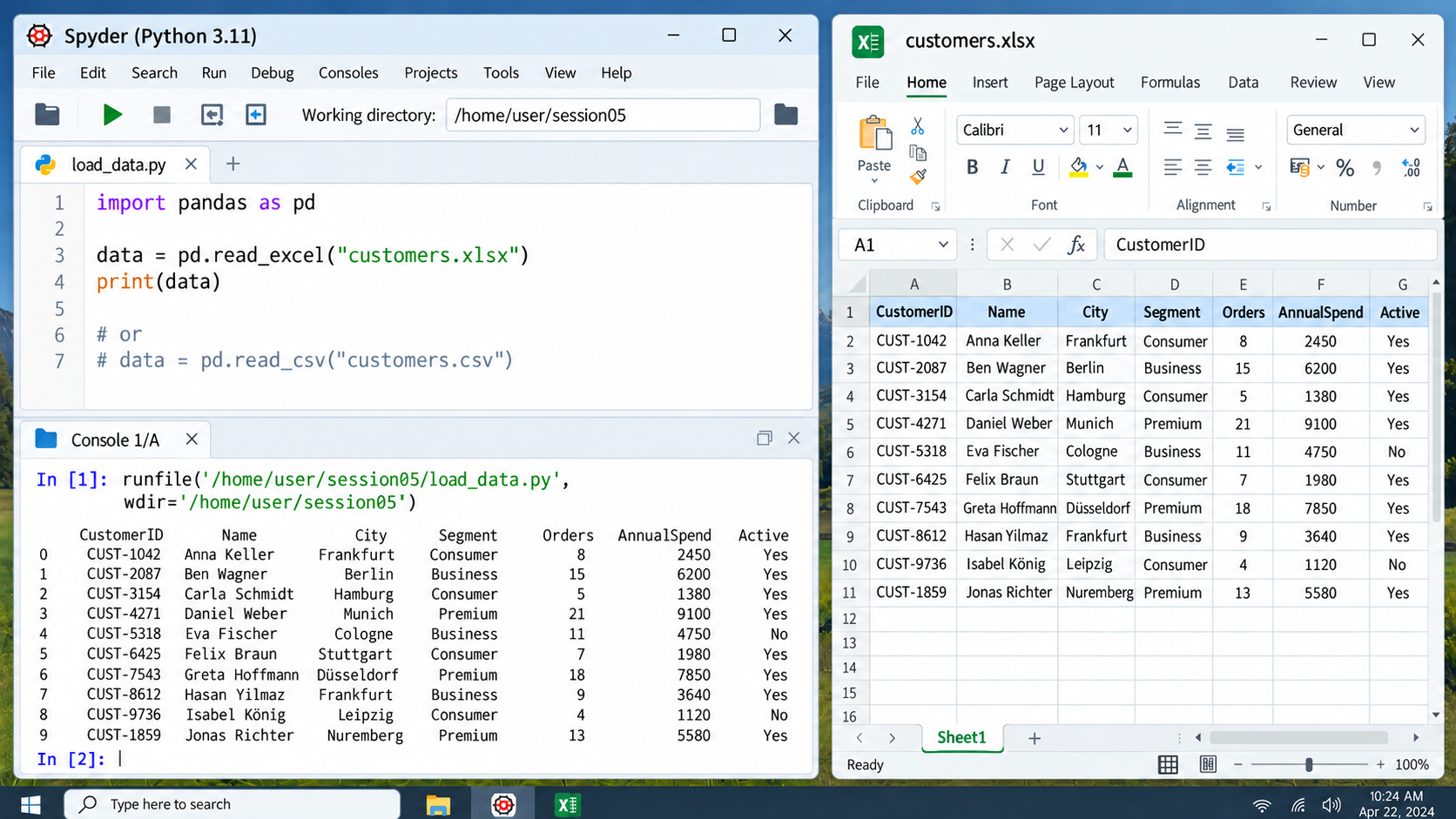
The running example is customers.xlsx.

customers = pd.read_excel('customers.xlsx')

Slide 26 — Position-based selection with `iloc` (integer location)

iloc selects values based on their position in the dataframe.

This is conceptually similar to referring to cells by their position in Excel. However, Python starts counting at 0 rather than 1.

First, try to access what we might intuitively consider the first cell:

customers.iloc[1, 1]

This does not return the first cell. Both row and column positions start at 0:

customers.iloc[0, 0]

The first argument identifies the row position and the second identifies the column position.

customers.iloc[0, :]    # first row, all columns
customers.iloc[:, 0]    # all rows, first column

The colon : means “all positions” along that dimension.

Slide 27 — Ranges and other `iloc` selections

As elsewhere in Python, ranges include the starting position but exclude the ending position.

For example, positions 2–4 correspond to the 3rd through 5th rows:

customers.iloc[2:5, :]
# Note: last element (5) is exclusive!

The same syntax can be used for columns:

customers.iloc[:, 1:4]

Negative positions count backwards from the end:

customers.iloc[:, -1]    # last column
customers.iloc[:, -2]    # second-to-last column
customers.iloc[-1, :]    # last row

Specific positions can also be supplied as lists:

customers.iloc[[0, 1, 2, 3, 4], [0, 3]]

Or ranges and lists can be combined:

customers.iloc[0:5, [0, 3]]

This selects the first five rows and columns at positions 0 and 3.

Why positions can be fragile

iloc always refers to the current position of rows and columns.

Suppose we want to send a goodie to the two customers who are currently inactive. Looking at the dataframe, they are currently in positions 4 and 8:

goodie_customers = customers.iloc[[4, 8], :]
goodie_customers

This works as long as the structure of the file remains exactly the same.

Imagine saving the script and leaving for lunch.

While we are away, somebody else edits customers.xlsx:

the customers are sorted differently;
an additional customer may be added;
columns may be inserted or rearranged.

After returning, we run exactly the same command:

customers = pd.read_excel('customers.xlsx')

goodie_customers = customers.iloc[[4, 8], :]
goodie_customers

The command still runs, but it may now select different customers or columns.

The positions have changed.

Transition: If observations and variables have meaningful names, it is usually safer to access them using these labels instead.

Slide 23 — Accessing columns by name

We have already seen that columns have names.

They can be inspected using:

customers.columns

A single column can be selected directly by its name:

customers['City']

Multiple columns can also be selected:

customers[['Name', 'City']]

Column names therefore already provide a label-based way of accessing data.

For rows, pandas can use meaningful labels as well.

Slide 24 — Giving rows meaningful labels

Our dataset contains a natural identifier for every observation: CustomerID.

We can tell pandas to use this variable as the row index when reading the file:

customers = pd.read_excel(
    'customers.xlsx',
    index_col='CustomerID'
)

Inspect the row labels:

customers.index

The dataframe now has two kinds of meaningful labels:

row labels such as CUST-1042;
column labels such as Name, City, and AnnualSpend.

loc uses these labels rather than integer positions.

customers.loc['CUST-1042', :]

Select one variable for this customer:

customers.loc['CUST-1042', 'Name']

Select particular columns:

customers.loc[
    'CUST-1042',
    ['Name', 'City', 'AnnualSpend']
]

Slide 25 — Selecting with `loc`

loc follows the same basic structure as iloc:

dataframe.loc[rows, columns]

The difference is that the arguments are labels rather than positions.

Select all customers and one column:

customers.loc[:, 'City']

Select several customers and columns:

customers.loc[
    ['CUST-1042', 'CUST-4271'],
    ['Name', 'City']
]

Label ranges are also possible:

customers.loc[
    'CUST-1042':'CUST-4271',
    'Name':'Segment'
]

Unlike iloc, the ending label is included for loc.

Therefore, both select four rows and three columns in the current dataframe:

customers.iloc[0:4, 1:4]
customers.loc[
    'CUST-1042':'CUST-4271',
    'Name':'Segment'
]

Note that label slices select everything between the two labels in the current index order. For robust identification of particular observations, explicit labels or conditions are preferable.

Illustrate that even label ranges are dependen on sort order: save file with different sorting and run again.

Slide 24/25 — Condition-based selection with `loc`

Often we do not know the identifiers of the observations we want beforehand.

Instead, we identify them using a condition.

For example, select all inactive customers:

customers.loc[customers['Active'] == 'No', :]

Or select only the information needed for sending the goodie:

goodie_customers = customers.loc[
    customers['Active'] == 'No',
    ['Name', 'City']
]
goodie_customers

This expresses what we actually want:

Select the customers whose Active value is No.

It does not depend on knowing their current positions.

Slide 29 — Labels remain meaningful after sorting

Consider one particular customer:

customers.loc[
    'CUST-5318',
    ['Name', 'AnnualSpend', 'Active']
]

Now change the order of the dataframe:

customers = customers.sort_values(by='AnnualSpend')
customers

The customer’s position has changed.

But the same label still identifies the same customer:

customers.loc[
    'CUST-5318',
    ['Name', 'AnnualSpend', 'Active']
]

The condition-based goodie selection also continues to work:

customers.loc[
    customers['Active'] == 'No',
    ['Name', 'City']
]

This is the central distinction:

iloc follows positions; loc follows labels.

Slide 28 — Comparing `loc` and `iloc`

Both methods use the structure

dataframe[rows, columns]

but interpret the arguments differently.

iloc uses integer positions:

customers.iloc[0, 1]
customers.iloc[0:4, 1:4]

loc uses labels:

customers.loc['CUST-1042', 'Name']

customers.loc[
    'CUST-1042':'CUST-4271',
    'Name':'Segment'
]

Important difference: Ranges in iloc vs. loc

There is also an important difference for ranges:

iloc[0:4] includes positions 0, 1, 2, and 3;
loc['CUST-1042':'CUST-4271'] includes both named endpoints.

Slide 29/30 — What if we do not specify a row index?

Compare reading the same file in two ways.

First, use CustomerID as the row index:

customers = pd.read_excel(
    'customers.xlsx',
    index_col='CustomerID'
)
customers
customers.index

Now read the file without specifying an index:

customers_default = pd.read_excel('customers.xlsx')
customers_default
customers_default.index

If we do not specify an index, pandas creates labels such as:

0, 1, 2, 3, ...

This can make loc and iloc initially look very similar:

customers_default.loc[0]
customers_default.iloc[0]

Both currently return the first row.

However, they still mean different things:

loc[0] means: select the row whose label is 0;
iloc[0] means: select the row currently in the first position.

The difference becomes visible after changing the row order:

customers_default = customers_default.sort_values(
    by='AnnualSpend'
)

customers_default.loc[0]
customers_default.iloc[0]

The automatically generated integer index is therefore a special case in which labels happen to look like positions.

For datasets with meaningful identifiers such as CustomerID, using these identifiers as the index makes the distinction much clearer.

Slide 31 — DataFrame selection

../materials/data/countries.csv

In-class exercise countries1.py

import pandas as pd

countries = pd.read_csv('data/countries.csv')

countries['Country']
countries.Country

countries.iloc[:, [0, 3]]
countries.iloc[1:5, 0:3]
countries.iloc[[11, 6, 14], [0, 3]]

countries.loc[:, ['Country', 'GDP']]
countries.loc[2:5, ['Country', 'GDP']]
countries.loc[4:13, ['Country', 'Continent', 'Area']]

Run countries.columns and countries.index to access the current column/row labels
Guide students through selecting columns and rows with iloc and loc.

Break — 10 minutes

Discuss solution of `contries1.py` exercise (> Previous page)

Slide 32 — Adding rows and columns

Rows can be added using a new row label. Because CustomerID is our index, we can use the identifier of the new customer directly.

customers.loc['CUST-9999'] = [
    'Alex Miller',
    'Frankfurt',
    'Business',
    12000,
    'Yes'
]
customers

Using a dictionary makes clear which value belongs to which column and does not depend on the current column order.

We can also create new columns from existing information. For example, convert annual spending into an approximate monthly value:

customers['MonthlySpend'] = customers['AnnualSpend'] / 12

Or create a column with the same value for every customer:

customers['Country'] = 'Germany'

The important distinction is that .loc[...] can add a row, whereas assigning to customers['...'] adds or replaces a column.

Slide 34 — Deleting rows and columns

drop() removes rows or columns by their labels.

Remove the customer we just added:

customers = customers.drop('CUST-9999')

Because rows are the default (axis=0), we do not need to specify an axis.

To remove one of our newly created columns:

customers = customers.drop('MonthlySpend', axis=1)
customers = customers.drop('Country', axis=1)

Here, axis=1 tells pandas that the labels refer to columns rather than rows.

drop() normally returns a modified DataFrame rather than changing customers automatically. We therefore assign the result back to customers.

Slide 35 — Sorting and useful DataFrame functions

We can sort customers according to one variable. For example, sort from lowest to highest annual spending:

customers_sorted = customers.sort_values(
    by='AnnualSpend'
)

customers_sorted

To show the highest-spending customers first:

customers_sorted = customers.sort_values(
    by='AnnualSpend',
    ascending=False
)

customers_sorted

Several columns can be used as sorting priorities:

customers_sorted = customers.sort_values(
    by=['Segment', 'AnnualSpend'],
    ascending=[True, False]
)

customers_sorted

This first groups customers by Segment and then orders customers within each segment from highest to lowest annual spending.

Slide 36 — Modifying and sorting data

../materials/data/countries.csv

In-class exercise countries2.py

import pandas as pd

countries = pd.read_csv('data/countries.csv')

countries.loc[len(countries)] = ['Belgium',11.5,11.849,803.166,'Europe']

countries.sort_values(by='Country')

countries['GDP_per_capita'] = countries.GDP / countries.Population

countries.sort_values(by='GDP_per_capita', ascending=False)

countries = countries.drop('GDP_per_capita', axis=1)

countries = countries.drop(20)

Summary and announcements

Questions for the Excel exam?

Notes for improvement

Take notes on improvements and common questions during the session and add them to feedback.qmd afterwards.

Preparation

Working directories and paths

Homework

Blackboard summary (develop with live demonstrations)

Setup to explain loc/iloc access

Slide 26 — Position-based selection with iloc (integer location)

Slide 27 — Ranges and other iloc selections

Slide 23 — Accessing columns by name

Slide 24 — Giving rows meaningful labels

Slide 25 — Selecting with loc

Slide 24/25 — Condition-based selection with loc

Slide 29 — Labels remain meaningful after sorting

Slide 28 — Comparing loc and iloc

Slide 29/30 — What if we do not specify a row index?

Slide 31 — DataFrame selection

Discuss solution of contries1.py exercise (> Previous page)

Slide 32 — Adding rows and columns

Slide 34 — Deleting rows and columns

Slide 35 — Sorting and useful DataFrame functions

Slide 36 — Modifying and sorting data

Summary and announcements

Slide 26 — Position-based selection with `iloc` (integer location)

Slide 27 — Ranges and other `iloc` selections

Slide 25 — Selecting with `loc`

Slide 24/25 — Condition-based selection with `loc`

Slide 28 — Comparing `loc` and `iloc`

Discuss solution of `contries1.py` exercise (> Previous page)