Machine Learning for Big Data

Machine Learning Baselines: Classification

Session 5 | 2026-09-17

• Understand how logistic regression uses a linear predictor and sigmoid function to produce probabilities, apply thresholds, and interpret log-odds and coefficients.
• Evaluate classification models using confusion matrices and metrics such as accuracy, precision, recall, and F1 score.
• Apply model predictions to decision-making by selecting appropriate thresholds based on business costs and expected value.

Business problem: Churn prediction

Predicting customer churn

A lost customer is often a predictable customer. Firms collect many traces of customer relationships — usage, spending, support interactions, contract data. The analytical challenge is to turn these traces into an early warning system.

Typical variables in a churn dataset

• Who is the customer? tenure, segment, contract type, subscription tier
• How do they use the service? login frequency, feature usage, inactivity days
• How satisfied are they? complaints, support tickets, response times, NPS/satisfaction
• Are there warning signs? payment delays, downgrades, cancellations of add-ons, price sensitivity

Geometric view of the problem

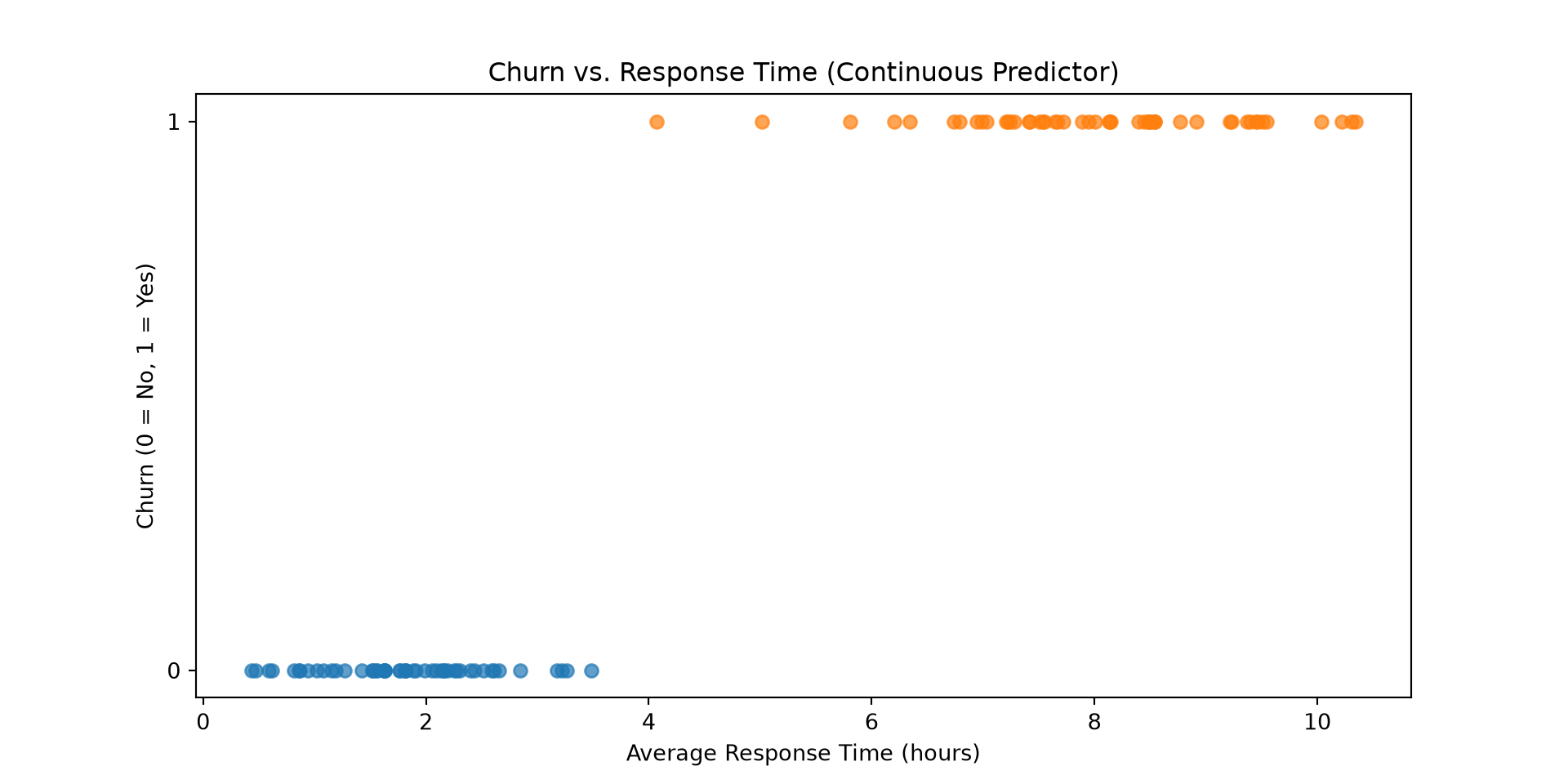
Churn prediction is a binary classification problem:

Possible approach: We could use Linear Regression with a threshold at 0.5 to classify output:

• If \(f(x) < 0.5\), predict y=0
• If \(f(x) \ge 0.5\), predict y=1

On whiteboard: draw previous versions (continuous -> continuous; categorical -> continuous / multidimensional)

• good (simple; geographical) explanation: https://www.youtube.com/watch?v=yIYKR4sgzI8
• TODO : include illustrations from video, min 2.17 and 3.20

Our natural expectation would be decreasing marginal effects - if customers are reasonably annoyed by waiting times, they will quit. There is no linear change with every additional hour they wait.

On slides: Draw regression line and illustrate the cutoff threshold when the y=0.5 cuts the regression line.

Illustrate sensitivity of regression lines to outliers (min 5 in https://www.youtube.com/watch?v=4u81xU7BIOc)

Also: linear regression will not respect the restriction of outcomes to {0,1}, but also give larger or negative (continuous) values. The “marginal effects” logic of linear regression does not make sense.

Logistic regression

General binary classification problems

Examples:

• Online transactions: Fraudulent (yes/no)?
• Customer churn: yes/no?
• EMail: Spam/not spam?

\[y \in \{0,1\}\] with

0: “Negative class” (e.g., no fraud, no churn, no spam)
1: “Positive class” (e.g., fraud, churn, spam)

Don’t be confused by Logistic “Regression” - it works like regression, but it is actually a classification algorithm

The binary classification can be extended to multiple classes:

\[y \in \{0,1,2,3,4\}\]

Logistic regression models

Ideally, our model should predict the probability of \(y_i=1\). This would allow us to apply a threshold for classification, but it would also give us more information (how likely an observation belongs to the positive class).

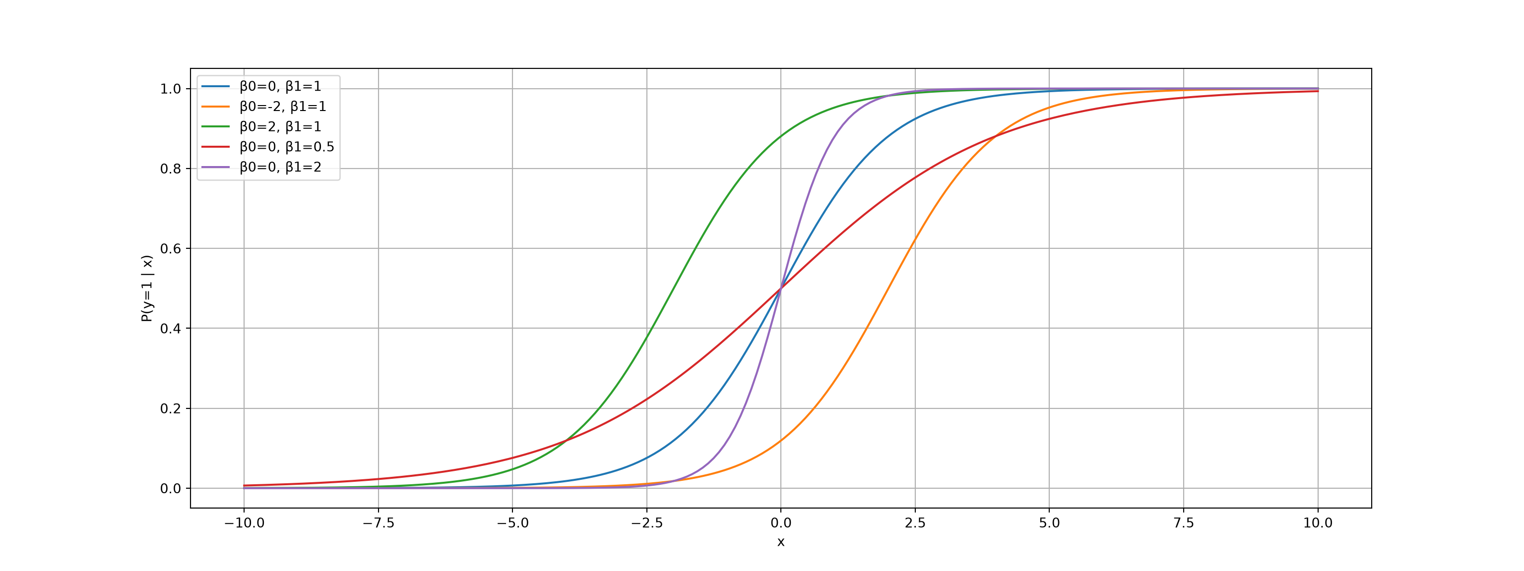
It means we need a model that produces predicted probabilities between 0 and 1:

Step 1: Linear model

\[z_i = \beta_0 + \beta_1 x_i\]

Step 2: Transform to probability via sigmoid function

\[\mathbb{P}(y_i = 1 \mid x_i) = \sigma(z_i) \text{ with } \sigma(z) = \frac{1}{1 + e^{-z}}\]

Logistic regression model

\[\mathbb{P}(y_i = 1 \mid x_i) = \frac{1}{1 + e^{-(\beta_0 + \beta_1 x_i)}}\]

• Linear predictor \(z\) → transformed by the sigmoid (logistic) function (output always in \([0,1]\))
• Can be interpreted as a probability (next slide)

Log-odds

Logistic regression assumes that the log-odds of the outcome are linear in the predictors:

\[\log\left(\frac{p_i}{1 - p_i}\right) = \beta_0 + \beta_1 x_i\]

Note: \(\frac{p_i}{1 - p_i}\) are the “odds”.

This implies a sigmoid-shaped relationship between \(x_i\) and the probability of \(y_i=1\):

\[p_i = \frac{1}{1 + e^{-(\beta_0 + \beta_1 x_i)}}\]

The sigmoid function serves as a link function to convert the linear predictor into a probability.

The Sigmoid function

Note

• Changing \(\beta_0\) shifts the curve left/right
• Changing \(\beta_1\) changes slope (flatter vs. steeper transition)

Highlight that the sigmoid function resolves the “constant marginal effects problem”

Estimation: Maximum likelihood

Instead of minimizing squared errors, logistic regression chooses parameters that make the observed data most likely.

Core idea: We want predicted probabilities to match observed outcomes:

• If \(y_i = 1\) → predicted probability should be high
• If \(y_i = 0\) → predicted probability should be low

Likelihood function

For each observation: \(P(y_i \mid x_i) = p_i^{y_i} (1 - p_i)^{1 - y_i}\)

For all observations:

\[L(\beta) = \prod_{i=1}^n p_i^{y_i} (1 - p_i)^{1 - y_i}\]

Maximization: Choose \(\beta_0, \beta_1\) to maximize this likelihood

Intuition: We search for the model that assigns high probability to what actually happened.

Logistic regression in R

We estimate the model using base R’s glm() function:

library(tidyverse)
library(broom)

df <- tibble(response_time=c(1,2,3,5,7,8,9,11), churn=c(0,0,0,0,1,1,1,1))

model <- glm(churn ~ response_time, data=df, family=binomial())
tidy(model)

# A tibble: 2 × 5
  term          estimate std.error statistic p.value
  <chr>            <dbl>     <dbl>     <dbl>   <dbl>
1 (Intercept)     -140.    306192. -0.000457   1.000
2 response_time     23.3    50231.  0.000465   1.000

Interpretation of coefficients

Logistic regression coefficients are not directly effects on probability. They describe effects on the log-odds.

Coefficient meaning

\[\log\left(\frac{p}{1-p}\right) = \beta_0 + \beta_1 x\]

• \(\beta_1\): change in log-odds when \(x\) increases by 1

Odds ratios: Exponentiate the coefficient

• \(e^{\beta_1}\) gives the multiplicative change in odds for a one-unit increase in \(x\).
• Example: \(1.5\) → odds increase by 50%; \(0.7\) → odds decrease by 30%.

Note: The effect on probability is nonlinear and depends on the starting probability.

Takeaway: Logistic regression is linear in log-odds — but nonlinear in probabilities.

→ Same change in \(x\) has different impact depending on where you are on the sigmoid curve

Evaluation

Predicted probabilities

A logistic regression model predicts a probability of churn:

\[ P(\text{churn}_i=1\mid x)=\frac{1}{1+e^{-(\beta_0+\beta_1 x_i)}} \]

A threshold (such as 0.5) is needed to convert probabilities into class labels.

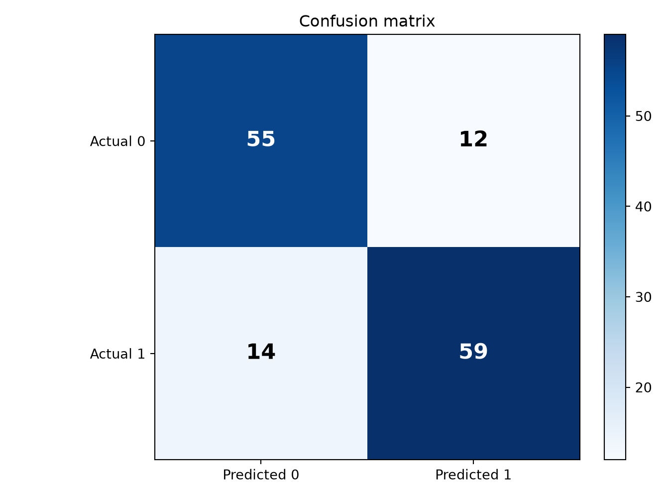
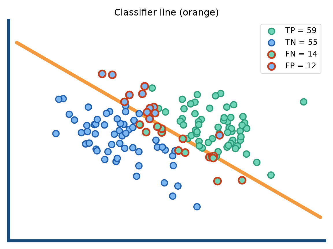
Comparing predicted vs. actual class labels allows us to evaluate the performance of a classifier like logistic regression.

Note: there are no meaningful residuals (or \(R^2\)), as in linear regression models.

Confusion matrix

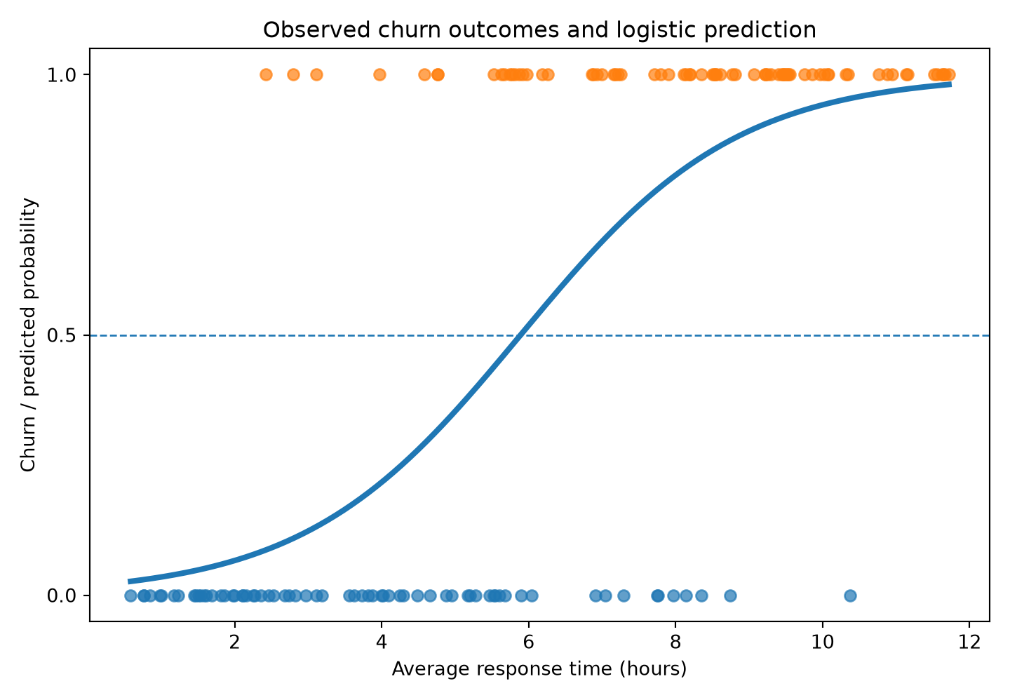
Using a 0.5 threshold, predicted probabilities are turned into classes.

The confusion matrix summarizes:

• True negatives (TN): predicted no churn, observed no churn
  
• False positives (FP): predicted churn, observed no churn
  
• False negatives (FN): predicted no churn, observed churn
  
• True positives (TP): predicted churn, observed churn

Evaluation metrics

Metric	Formula	Interpretation
Accuracy	\(\frac{TP+TN}{TP+TN+FP+FN}\)	Overall share of correct predictions
Precision	\(\frac{TP}{TP+FP}\)	Among predicted positives, how many are actually positive?
Recall	\(\frac{TP}{TP+FN}\)	Among actual positives, how many did the model identify?
F1	\(2\cdot\frac{\text{Precision}\cdot\text{Recall}}{\text{Precision}+\text{Recall}}\)	Balance between precision and recall

The metrics depend on how we define the classes (what is “positive”).

ROC curve and AUC

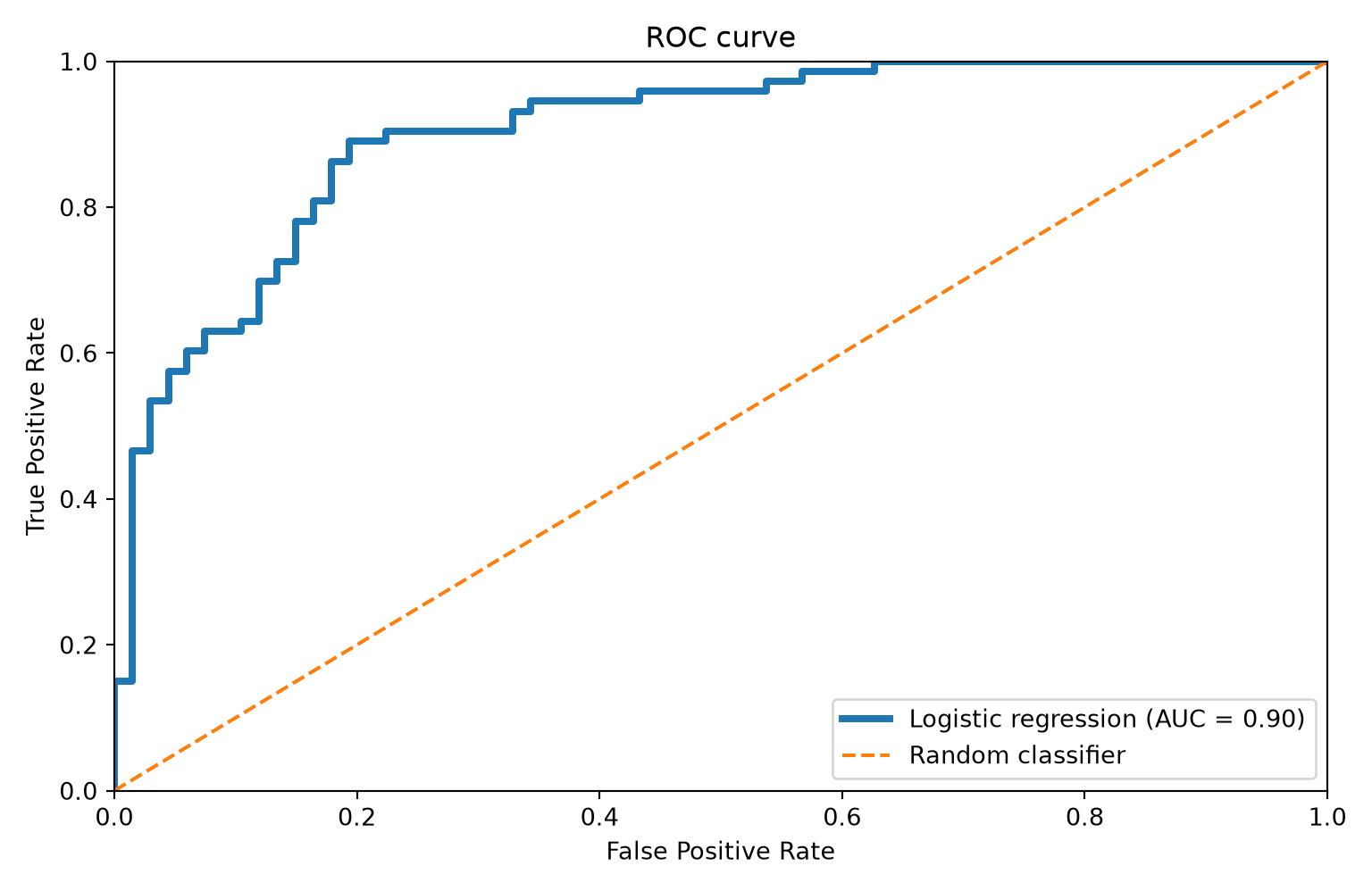
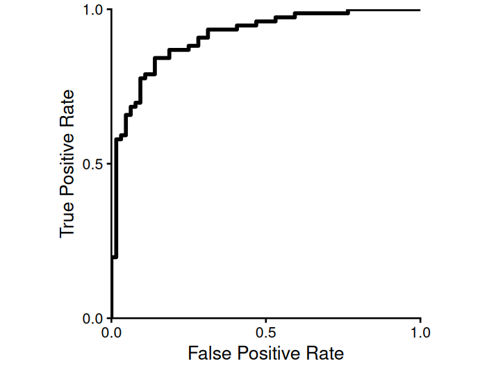
The Receiver Operating Characteristic (ROC) curve summarizes the trade-off between:

• True Positive Rate (aka. recall or sensitivity)
• False Positive Rate

As we vary the classification threshold, the model becomes more or less conservative in predicting churn = 1.

Area under the curve (AUC) summarizes ROC performance in a single number:

• AUC = 0.5: no better than random guessing
• AUC = 1.0: perfect separation

A good classifier achieves:

• high true positive rate
• low false positive rate

→ Curves closer to the top-left corner indicate better model fit.

Unlike accuracy, ROC/AUC evaluates the classifier across all possible thresholds.

Emphasize that each point on the ROC curve corresponds to a different classification threshold.

Good link back to the confusion matrix:

• lowering the threshold catches more churners
• but also creates more false alarms

AUC is especially useful when we want to compare models independently of one specific cutoff such as 0.5.

ROC and AUC in R

Calculate ROC and AUC

library(pROC)

# the model object is the
# fitted classifier providing predictions
pred <- predict(model, type = "response")

roc_obj <- roc(
  df$churn,       # Ground truth
  pred,           # Prediction
  levels = c(0, 1),
  direction = "<" # Higher scores:= class 1
)

auc(roc_obj)

Area under the curve: 0.9114

Plot ROC curve

library(ggplot2)

roc_df <- data.frame(
  fpr = 1 - roc_obj$specificities,
  tpr = roc_obj$sensitivities
)

roc_plot <- ggplot(roc_df, aes(fpr, tpr)) +
  geom_path(linewidth = 1)

How does roc() work?

function roc(actual, scores, levels, direction):

    # Identify actual positive and negative cases
    negative = actual == levels[0]
    positive = actual == levels[1]

    for threshold in thresholds(scores):

        # direction specifies the ordering of ground-truth scores
        # "<": negatives have lower scores than positives
        # ">": negatives have higher scores than positives
        if direction == "<":
            predicted = scores >= threshold
        else:
            predicted = scores <= threshold

        # Evaluate predictions against actual outcomes and store in roc_object
        TP = count(predicted & positive)
        FP = count(predicted & negative)
        TPR = TP / count(positive)
        FPR = FP / count(negative)

    return roc_object # (containing TPR, FPR, ...)

Key takeaway:

• levels: Which actual outcome is positive?

• direction: Which side of the threshold predicts positive?

• levels: First = controls (negative class); second = cases (positive class).

• direction = "<": Controls have lower scores; higher scores predict positive.

• direction = ">": Controls have higher scores; lower scores predict positive.

This is conceptual pseudocode; pROC uses cumulative counts rather than calculating a separate confusion matrix at each threshold.

For levels: Consider prediction of defaults vs. pays back.

From prediction to decisions

From prediction to decision

A logistic regression model predicts a probability of churn:

\[ p(x) = P(\text{churn}=1 \mid x) \]

This probability is based on historical data, reflecting how similar customers behaved in the past, and capturing a baseline churn risk. It is not a certainty.

Suppose a firm has two possible actions:

• Intervene: offer a retention incentive
• Do nothing

So the business problem is no longer only:

Who is likely to churn?

It becomes:

For whom is an intervention worth it?

Important distinction: The model predicts what is likely to happen if we do nothing different. It does not yet tell us whether we should intervene.

Decision-making under uncertainty

We can use the expected value criterion to translate predictions into decisions by combining:

• Probability of churm predicted by the model
• Business consequences of the action

A simple payoff structure:

Action	Customer would churn	Customer would stay
Intervene	+20	-10
Do nothing	-100	0

Interpretation:

• Saving a likely churner creates value
• Intervening with a customer who would stay creates unnecessary cost
• Missing a true churner is very costly

Stress that these are simplified business values. They encode the firm’s priorities and economics.

Expected value of (not) intervening

Action	Customer would churn	Customer would stay
Intervene	+20	-10
Do nothing	-100	0

Probabilities:

• With probability \(p(x)\), the customer is at risk and intervention helps
• With probability \(1-p(x)\), the customer would stay anyway and intervention wastes resources

If we intervene, the expected value is:

\[EV(intervene) = p(x)\cdot 20 + (1-p(x))\cdot (-10) = 30p(x) - 10\]

If we do nothing, the expected value is:

\[ EV(do\_nothing) = p(x)\cdot (-100) + (1-p(x))\cdot 0 = -100p(x) \]

Interpretation:

• If the customer would churn, the firm bears a large loss
• If the customer would stay, there is no cost

Based on Elkan (2001).

Optimal decision rule

Instead of selecting one action, we should intervene whenever:

\[ EV(intervene) > EV(do\_nothing) \]

Insert the expected values:

\[ 30p(x) - 10 > -100p(x) \]

Simplify:

\[ 130p(x) > 10 \]

\[ p(x) > 0.077 \]

Decision threshold

This gives a clear rule:

Intervene if \(p(x) > 0.077\) (if predicted churn probability exceeds 7.7%).

The threshold is low because:

• Losing a customer is very costly
• Intervening is relatively cheap

So even a small churn probability can justify action.

A classification threshold does not have to be 0.5. It should depend on the business context.

This is a nice place to contrast statistical classification with managerial decision-making. Students often assume 0.5 is automatic or “correct”.

Two sources of knowledge

This decision combines two complementary inputs:

1. Data-driven component

• Logistic regression estimates: \[ p(x)=P(\text{churn}=1\mid x) \]

• Learned from historical data
  

• Provides a probability (what is likely to happen)

2. Business-driven component

• A threshold that determines when to act
  
• Ideally derived from expected value considerations
  
• Based on business costs, strategy, and domain knowledge

Summary

• Logistic regression is a method for binary classification, where the goal is to predict whether an outcome occurs (e.g., churn vs. no churn).
• It predicts probabilities \(P(y=1 \mid X)\) using a linear predictor combined with a sigmoid function, ensuring outputs between 0 and 1.
• Coefficients are interpreted in terms of log-odds (or odds ratios), not direct probability changes.
• Parameters are estimated via maximum likelihood, aiming to match predicted probabilities with observed outcomes.
• Model performance is evaluated using classification metrics such as confusion matrices, accuracy, precision, recall, F1, and ROC/AUC.
• A threshold is required to convert probabilities into class labels, and should be chosen based on business costs, not fixed at 0.5.

Feedback

Please take 1–2 minutes to reflect on today's session.

Complete the short feedback survey

References

Elkan, Charles. 2001. “The Foundations of Cost-Sensitive Learning.” International Joint Conference on Artificial Intelligence 17: 973–78. https://doi.org/10.5555/1642194.1642224.