Machine Learning for Big Data

Exploratory Data Analysis

Session 3 | 2026-09-11

• Describe variables, relationships between variables, and underlying structure in the data (e.g., clusters).
• Explore data sets using appropriate descriptive and visual techniques.
• Explain the role of exploratory data analysis in business decision-making.

Foundations

People are not very good at looking at a column of numbers or a whole data table and then determining important characteristics of the data. EDA techniques have been devised as an aid in this situation.

The following forms of EDA are typically distinguished:

	Univariate	Multivariate
Non-graphical	mean, median frequencies	cross-tabs correlations
Graphical	histograms dot plots	scatter plots clustering

Univariate exploratory data analysis

Descriptive statistics

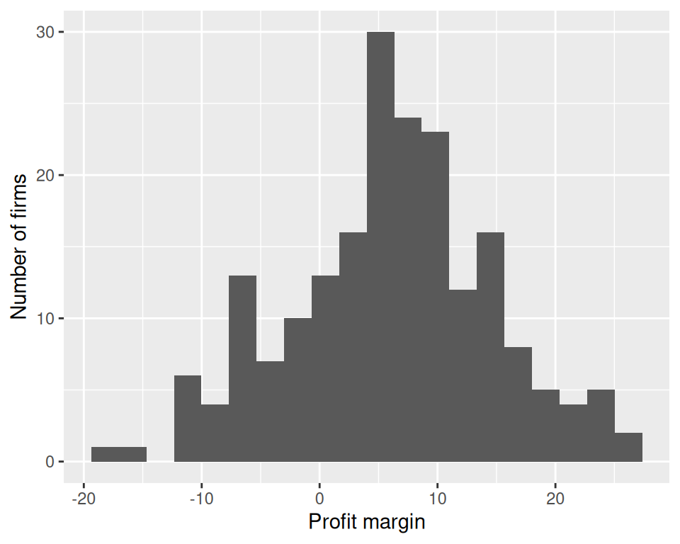
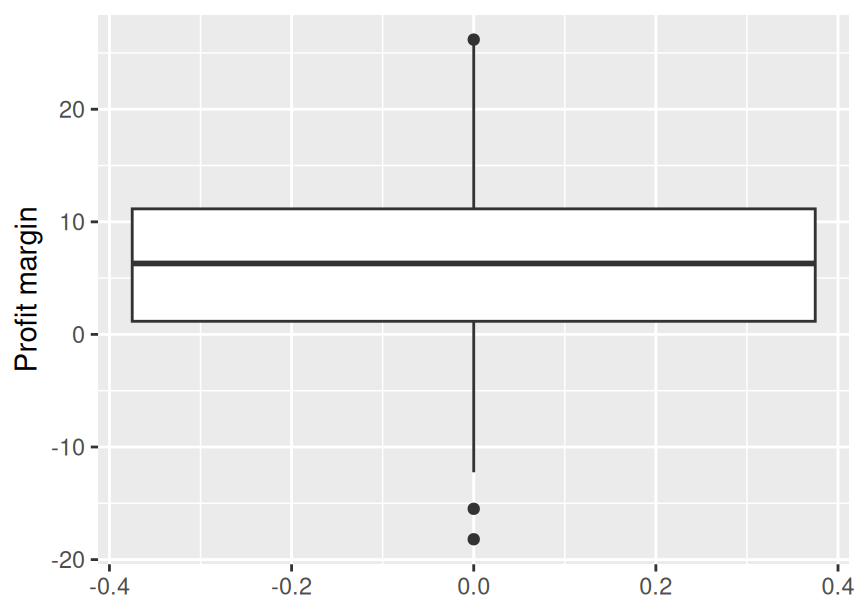
We use one real data set throughout the examples: 200 firms from four sectors.

library(tidyverse)

firm_data_df <- read_csv(
  paste0(
    "https://raw.githubusercontent.com/fs-ise/",
    "machine-learning-for-big-data/main/",
    "exercises/data/firm_data.csv"
  ),
  show_col_types = FALSE
)

head(firm_data_df)

# A tibble: 6 × 8
  company_id sector     revenue profit_margin growth_rate debt_ratio market_cap
  <chr>      <chr>        <dbl>         <dbl>       <dbl>      <dbl>      <dbl>
1 FIRM-0095  Healthcare   2118.        13.4          6.05      0.556     12427.
2 FIRM-0015  Healthcare    458.        10.1         21.5       0.350      5779.
3 FIRM-0030  Industry      464.         4.13        13.2       0.356      4452.
4 FIRM-0158  Finance       348.         9.57        16.1       0.472      3257.
5 FIRM-0128  Tech          804.         0.165       -3.35      0.761      1825.
6 FIRM-0115  Healthcare    845.        -4.47         1.11      0.729       790.
# ℹ 1 more variable: rd_intensity <dbl>

Descriptive statistics by variable type

Categorical variables (sector)

• frequency → number of observations per category

Numerical variables (profit_margin)

• mean → center
• variance / standard deviation → spread
• quantiles → position in the distribution
• compact overview of minimum, quartiles, median, mean, and maximum

table(firm_data_df$sector)

   Finance Healthcare   Industry       Tech 
        52         55         44         49 

mean(firm_data_df$profit_margin)

[1] 6.038353

var(firm_data_df$profit_margin)

[1] 74.06978

sd(firm_data_df$profit_margin)

[1] 8.60638

quantile(firm_data_df$profit_margin)

        0%        25%        50%        75%       100% 
-18.193454   1.165900   6.300245  11.151334  26.183842 

summary(firm_data_df$profit_margin)

   Min. 1st Qu.  Median    Mean 3rd Qu.    Max. 
-18.193   1.166   6.300   6.038  11.151  26.184 

Histogram: shape, center, and spread

• Numerical values are divided into intervals (bins).
• Bar height indicates how many observations fall into each interval.
• A histogram reveals the distribution’s shape, center, spread, and unusual observations.

ggplot(firm_data_df, aes(x = profit_margin)) +
  geom_histogram(bins = 20) +
  labs(
    x = "Profit margin",
    y = "Number of firms"
  )

See ggplot2 documentation and cheatsheet.

Boxplot

• The boxplot is a condensed illustration of a distribution

• It consists of

  • Median (thick line)
  • 25% / 75% percentiles
  • “Whiskers”: the quartiles \(\pm 1.5 \times \mathrm{IQR}\)
  • Outliers that are higher/lower than the whiskers

ggplot(firm_data_df, aes(y = profit_margin)) +
  geom_boxplot() +
  labs(
    x = NULL,
    y = "Profit margin"
  )

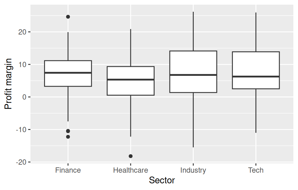
Boxplots can be used to compare different distributions

The same summary can be calculated for each category.

Observation: Industry and Tech have wider interquartile ranges than Finance. Finance has the highest median profit margin and several potential outliers.

ggplot(
  firm_data_df,
  aes(x = sector, y = profit_margin)
) +
  geom_boxplot() +
  labs(
    x = "Sector",
    y = "Profit margin"
  )

Multivariate exploratory data analysis

Multivariate non-graphical EDA

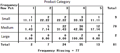
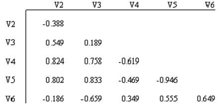
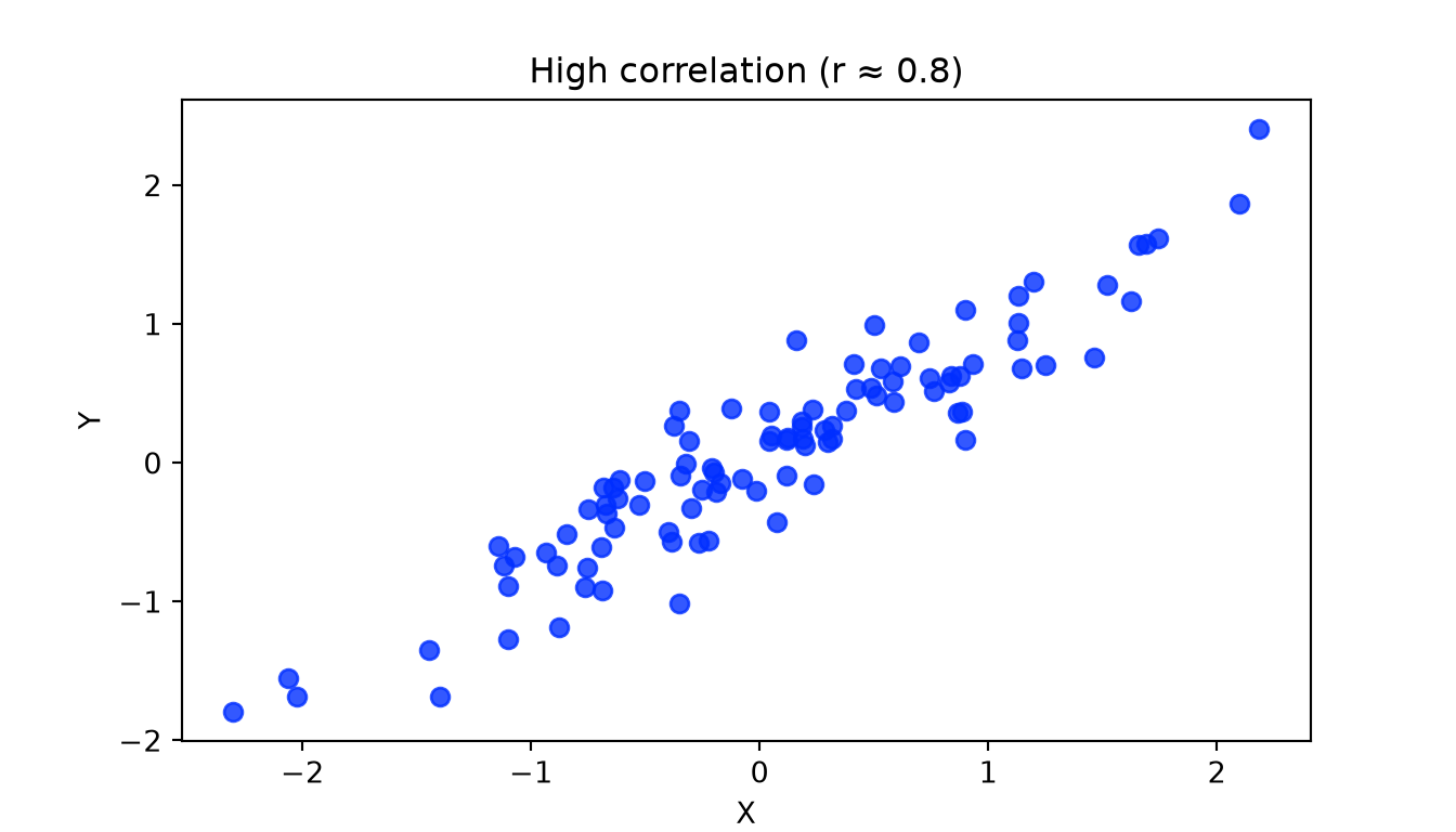
Multivariate non-graphical EDA techniques generally show the relationship between two or more variables in the form of either cross-tabulation for categorical variables or correlation statistics for numerical variables.

Multivariate graphical EDA

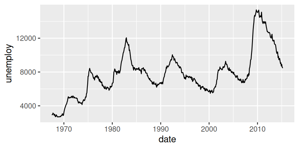
When exploring multiple variables together, the appropriate visualization depends on the types of variables being compared.

Scatterplot

ggplot(firm_data_df) +
  geom_point(
    aes(
      x = rd_intensity,
      y = profit_margin
    )
  )

Line plot

ggplot(economics) +
  geom_line(aes(x = date, y = unemploy))

Bivariate statistics: Correlation

Correlation measures how strongly two variables move together. Suppose we observe two variables for the same observations:

\[X = (x_1, x_2, ..., x_n)\]

\[Y = (y_1, y_2, ..., y_n)\]

The Pearson correlation coefficient is calculated as:

\[r = \frac{\sum_{i=1}^{n}(x_i-\bar{x})(y_i-\bar{y})} {\sqrt{\sum_{i=1}^{n}(x_i-\bar{x})^2}\sqrt{\sum_{i=1}^{n}(y_i-\bar{y})^2}}\]

Correlation vs. causality

Correlation: Two data series behave “similar”

Causality: Principle of cause and effect

Correlation does not imply causation.

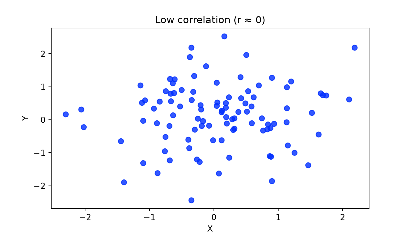
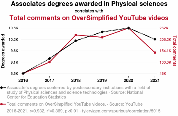
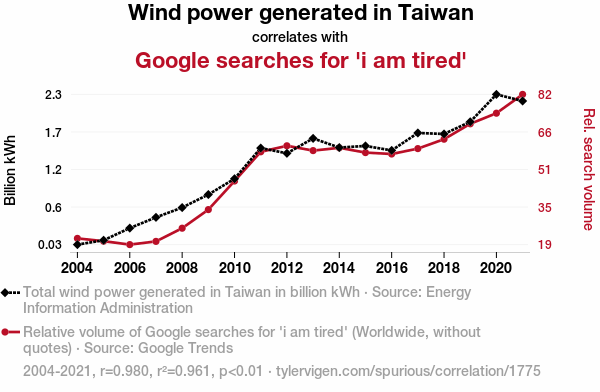
Bivariate correlations are often insufficient for prediction or explanation, requiring more powerful analytical models.

If causal explanations are unavailable, decisions may need to rely on predictions.

More examples are available at: https://www.tylervigen.com/spurious-correlations

Clustering in EDA

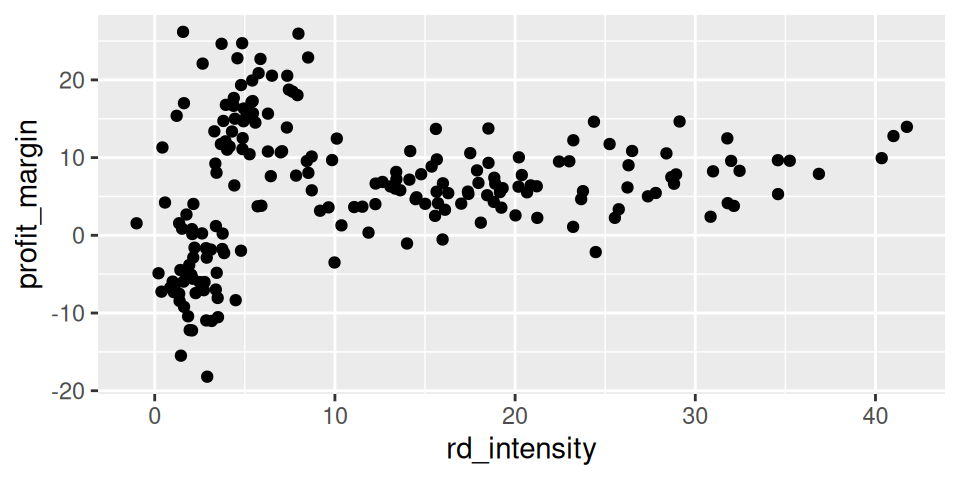
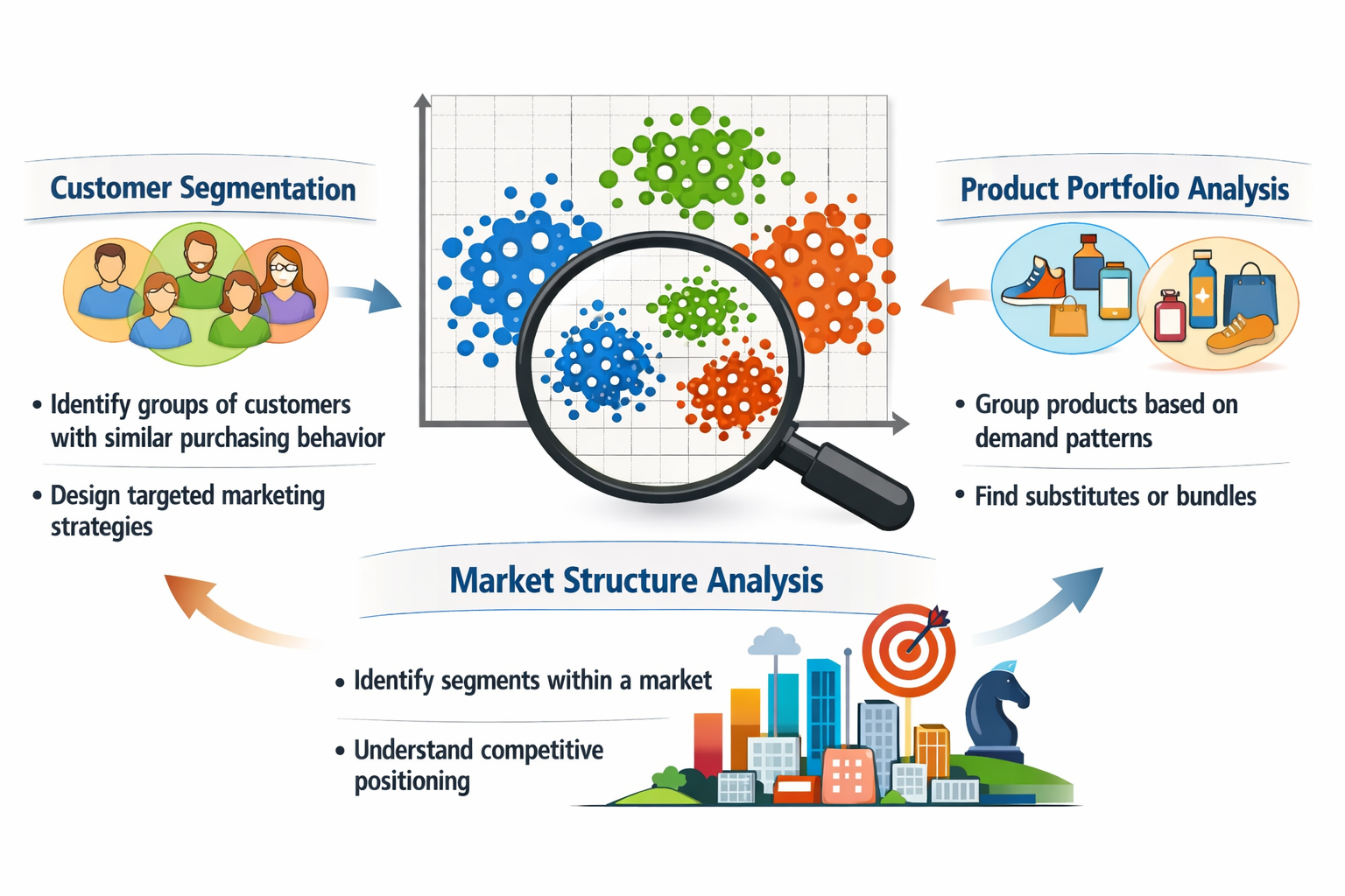
In multivariate exploratory data analysis, we often want to understand whether observations form natural groups.

Clustering is an EDA technique that groups similar observations based on their characteristics.

Common use cases include:

Timing: ~4 minutes.

Emphasize: clustering is usually not the final model. It is used to understand structure in the data.

Typical workflow:

EDA → clustering → interpretation → downstream analytics.

Families of clustering methods

Clustering algorithms can be grouped into several families of approaches.

Family	Examples	Key characteristics
Partitioning methods	k-means, k-medoids (PAM), bisecting k-means	divide observations into a predefined number k of clusters; k-means is computationally efficient and widely used for business/customer segmentation
Hierarchical methods	Agglomerative clustering, divisive clustering	clusters formed through successive merging or splitting; produce dendrograms (cluster trees); useful for exploratory structure discovery
Density-based methods	DBSCAN, HDBSCAN	clusters defined as regions of high density; identify arbitrary shapes and outliers/noise
Probabilistic / model-based methods	Gaussian mixture models	clusters modeled as probability distributions; allow soft cluster membership when groups overlap

In this lecture we focus on k-means (segmentation) and agglomerative hierarchical clustering.

Timing: ~5 minutes.

Goal: give students a quick mental map of clustering methods.

Emphasize that many algorithms exist, but we focus on the two most intuitive and widely taught ones:

• k-means
• agglomerative hierarchical clustering.

Segmentation clustering

Segmentation methods divide observations into k clusters.

Goal:

• maximize similarity within clusters
• maximize differences between clusters

The most widely used algorithm:

k-means clustering

Key assumption:

clusters are roughly spherical and similar in size.

Timing: ~2 minutes.

Explain the intuition first before showing the algorithm.

k-means: The algorithm

For a given k, the algorithm finds cluster centers that minimize within-cluster sum of squares.

Steps:

Randomly assign data points to k clusters

Repeat:

    calculate centroids for each cluster

    for each data point:
        compute distance to all centroids

        if x is not closest to its current centroid:
            assign x to the nearest centroid

    if centroids and cluster assignments no longer change:
        stop

Strengths: fast and scalable, easy to interpret

Limitations: must choose k, sensitive to scaling and outliers.

Timing: ~4 minutes.

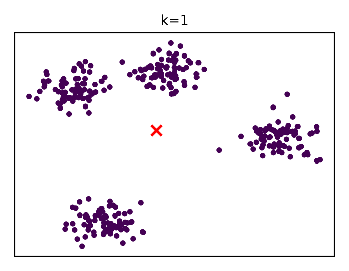
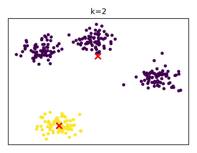
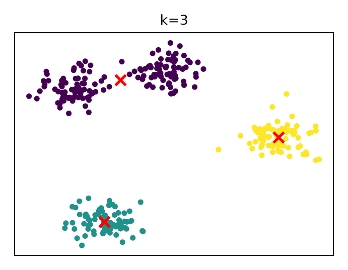
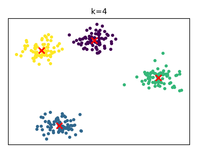
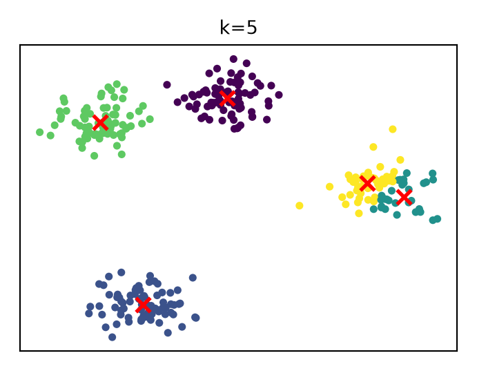
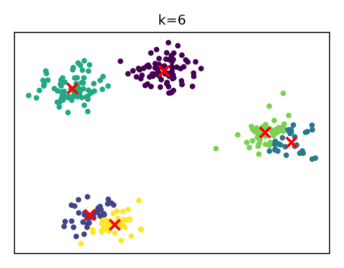
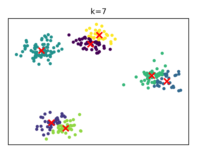
k-means: Comparison of solutions for different k

…

Note: The plots show the final result after the algorithm has converged, i.e., once observation assignments and cluster centroids no longer change.

k-means: Implementation in R

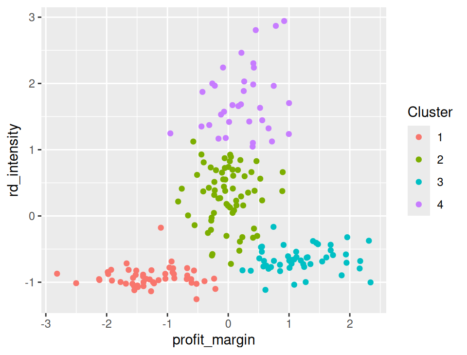
set.seed(42)       # for reproducibility

X <- firm_data_df |>
  select(profit_margin, rd_intensity) |>
  scale()

km <- kmeans(X, centers = 4, nstart = 25)

as.data.frame(X) |>
  mutate(cluster = factor(km$cluster)) |>
  ggplot(aes(x = profit_margin, y = rd_intensity, color = cluster)) +
    geom_point() + labs(color = "Cluster")

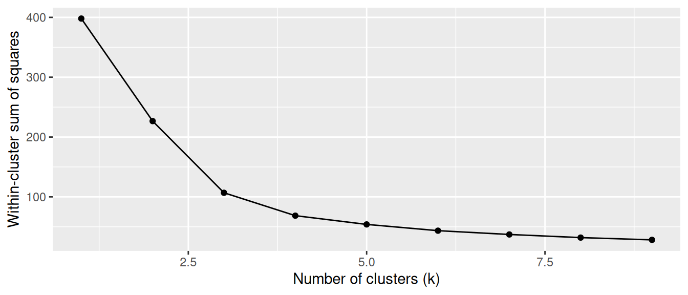
k-means: Choosing the number of clusters (I)

A common heuristic is the elbow method.

Idea:

• increase k
• measure improvement in model fit
• look for point where improvement slows

Example metric: within-cluster variance (inertia)

Choose k at the “elbow” (diminishing returns)

Timing: ~3 minutes.

Key point: inertia always decreases → we look for where gains flatten out.

Emphasize: heuristic, not a strict rule.

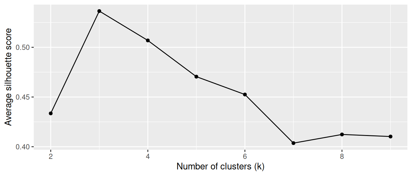
k-means: Choosing the number of clusters (II)

An alternative is the silhouette score.

Idea:

• evaluate cohesion (within clusters)
• evaluate separation (between clusters)
• combine both into a single score

Choose k that maximizes the score

Higher = better separation and compactness

Contrast with elbow:

• elbow → diminishing returns
• silhouette → clear maximum

Highlight: combines two criteria (cohesion + separation).

Hierarchical clustering

Hierarchical clustering builds a tree of clusters.

There are two types of hierarchical cluster methods:

• Agglomerative hierarchical clustering is a bottom-up clustering method. It starts with every single data object in a single cluster. Then, in each iteration, it agglomerates (merges) the closest pair of clusters by satisfying some similarity criteria, until all the data is in one cluster.
• Divisive hierarchical clustering is a top-down clustering method. It works similarly to agglomerative clustering but in the opposite direction. This method starts with a single cluster containing all data objects, and then successively splits resulting clusters until only clusters of individual data objects remain.

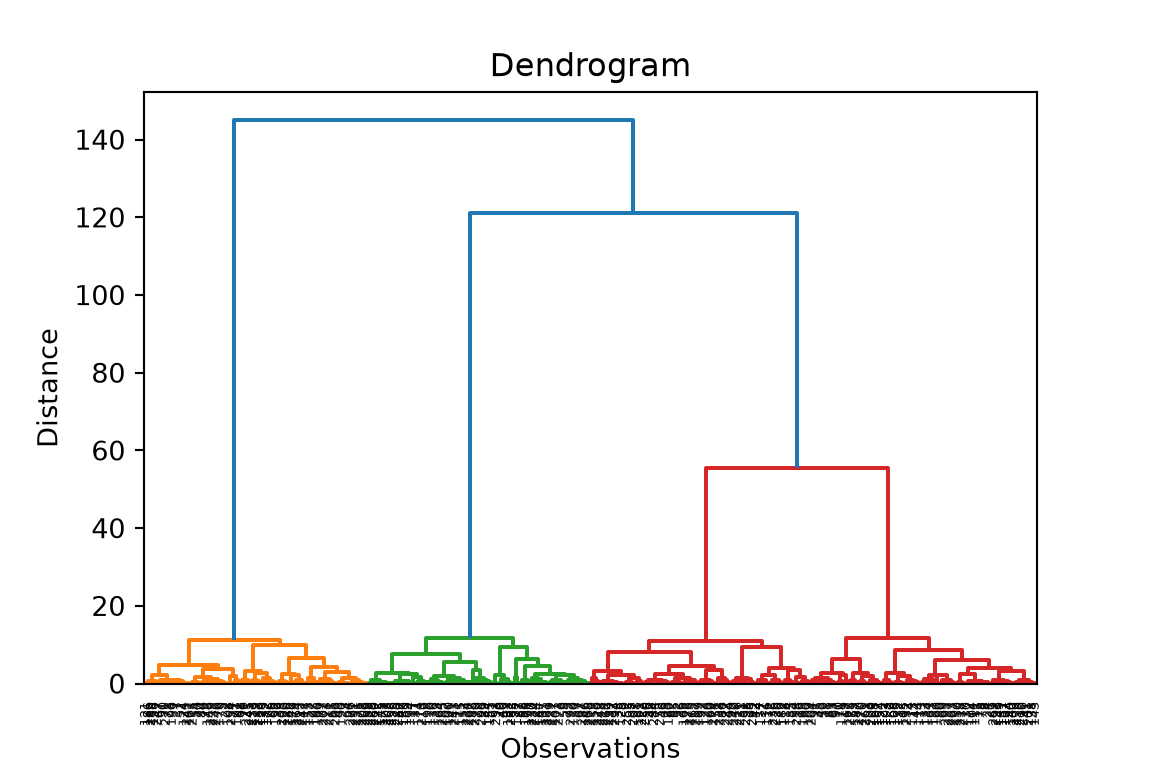
Dendrogram

A dendrogram is a tree diagram frequently used to illustrate the arrangement of the clusters produced by hierarchical clustering. The y-axis represents the value of this distance metric (e.g. Euclidean distance) between the clusters.

In a dendrogram the widths of the horizontal lines give an impression about the dissimilarity of the merging object. Thus, a good cluster number might be at a point from where the width of the following horizontal lines is significantly shorter.

This allows us to explore clusters at multiple levels of granularity.

Evaluation of clusters

⚠ Clustering algorithms will always produce groups, even when no meaningful structure exists.

Therefore, clusters must be evaluated.

Common evaluation approaches include:

• internal validation

  • silhouette score
  • cluster stability

• external validation

  • compare with known labels or metadata

• interpretability checks

  • do cluster profiles make sense in the given context?

Timing: ~3 minutes.

Key warning:

Clusters \(\neq\) truth. They are hypotheses about structure in the data.

Based on Balijepally et al. (2011).

Why clustering is useful in analytics workflows

Clustering often supports later analytical steps.

For example:

• Customer segments in data warehouses

  • segments stored as features for reporting or dashboards

• Heterogeneity in regression models

  • different segments may follow different behavioral patterns
  • subgroup analysis or separate models

• Machine learning pipelines

  • clustering can generate features or latent groups

• Hypothesis generation and model development

  • clusters can reveal previously unnoticed patterns or structures
  • these patterns may suggest new hypotheses about behavior or relationships in the data
  • clustering can therefore inform model specification, variable selection, or interaction terms

Timing: ~3 minutes.

Key message: Clustering often produces insights that guide later modeling.

Summary

Exploratory Data Analysis (EDA) helps us understand data before modeling.

Key steps:

• Describe variables
  • univariate statistics (mean, variance, distributions)
  • visualization (histograms, boxplots)
• Analyze relationships
  • multivariate patterns (correlation, scatterplots)
  • ⚠ correlation \(\neq\) causation
• Identify structure
  • segmentation (elbow method/silhouette score)
  • hierarchical clustering (dendrogram)

EDA is not the final analysis, but a foundation for model building, decision-making, and hypothesis generation.

Feedback

Please take 1–2 minutes to reflect on today's session.

Complete the short feedback survey

References

Balijepally, VenuGopal, George Mangalaraj, and Kishen Iyengar. 2011. “Are We Wielding This Hammer Correctly? A Reflective Review of the Application of Cluster Analysis in Information Systems Research.” Journal of the Association for Information Systems 12 (5): 1. https://doi.org/10.17705/1JAIS.00266.