Machine Learning for Big Data

Analytics and Data Preparation

Session 2 | 2026-09-04

• Explain how computing power, algorithms, and analytics processes enabled modern machine learning and AI for big data.
• Compare data warehouse, data lake, and logical data warehouse architectures.
• Distinguish descriptive, predictive, and prescriptive analytics.
• Describe the CRISP-DM analytics process.
• Structure, clean, integrate, and transform data for analysis.
• Explain tidy-data principles and select appropriate data types.

Why did machine learning become so powerful?

Modern machine learning and AI for big data became powerful through three mutually reinforcing developments:

1. More computing power make it possible to process large datasets and train more demanding models.
2. New algorithms enable more powerful analytical models and new application areas.
3. New architectures optimize data processing and computation.
4. New analytics processes make analytical work more mature, pervasive, and standardized.

Computing power

Growth of computing power

The rapid acceleration of computing power—driven by advances in hardware, cloud infrastructure, and parallel processing—has enabled modern analytics and machine learning to scale to massive datasets.

Evolution of computing power

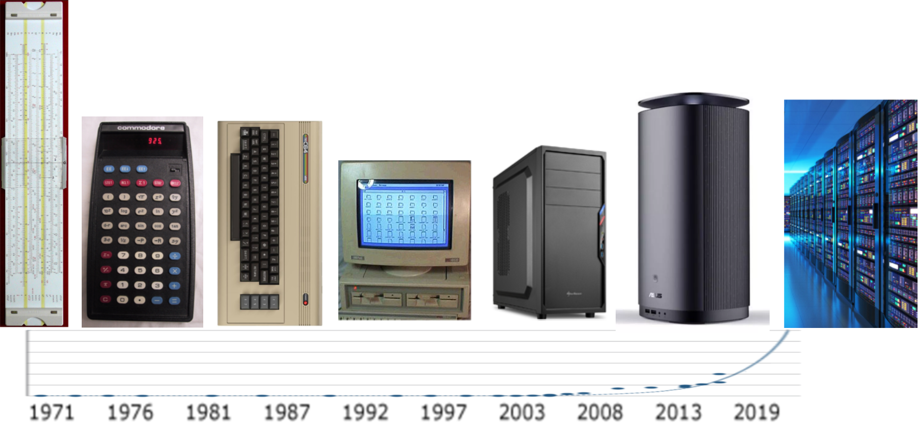
The growth of modern analytics is enabled by changing strategies for increasing computing power.

Era	Main strategy	Explanation
1970s–2000s (*)	Moore’s Law & miniaturization	Smaller transistors → more components per chip → faster processors
2005–today	Parallel computing	Performance increases by using multiple processors simultaneously
2010s–today	Specialized hardware	Chips optimized for specific workloads (GPUs, TPUs, AI accelerators)
Emerging	New computing paradigms	Alternative computing models such as quantum computing

(*) Miniaturization continues today, but progress has slowed as transistors approach physical limits. Advances such as extreme ultraviolet (EUV) lithography are required to continue scaling. See how $400 million machines are constructed to build modern chips: https://www.youtube.com/watch?v=MiUHjLxm3V0.

New algorithms

Algorithms

An algorithm is a step-by-step procedure for performing a computation and thereby solving a problem.

Algorithms determine which problems computers can solve and how efficiently they can solve them.

Examples:

• Dijkstra’s Shortest-Path Algorithm (1959) — Efficiently finding shortest paths through networks, foundational to routing, navigation, and network optimization
• Evolutionary Algorithms (1960s) — Population-based search and optimization methods inspired by evolution, used to find good solutions to complex problems where exact optimization is difficult
• Scheduling Algorithms (1990s–present) — Efficient process scheduling enabling operating systems to run tasks concurrently
• PageRank (1998) — Algorithm ranking webpages based on link structure, enabling scalable web search
• Deep Learning (2010s) — Improved neural network training enabling major advances in vision, speech, and language AI
• Gradient Boosting (2014) — High-performance ensemble learning algorithm widely used in predictive analytics and data science
• Transformer Models (2017–present) — Transformer architecture enabling large language models and generative AI

Algorithms enable more powerful analytical models

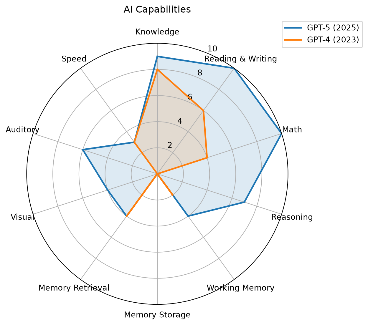
Traditional Regression

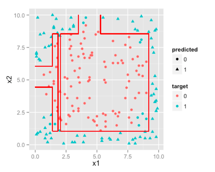
Decision Tree

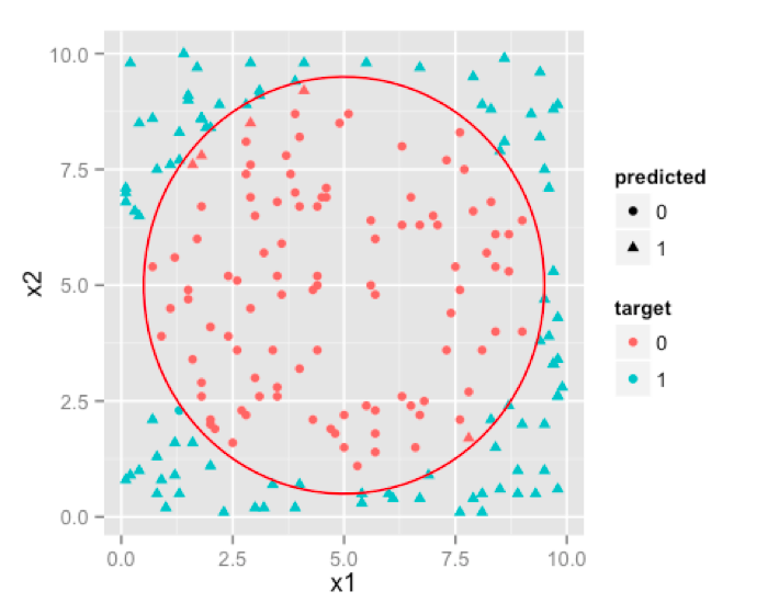
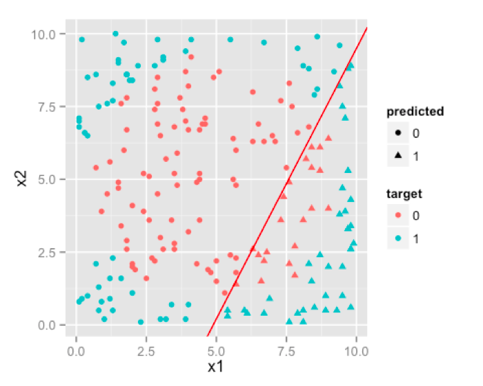
Neural Network

Algorithmic and analytical models across disciplines

There is a broad repertoire of models and methods from multiple disciplines, each with its own assumptions, data preparation steps, and modeling processes. While these fields often focus on methodological development, business analytics emphasizes applying these approaches to support understanding and decision-making in organizational contexts.

Discipline	Model culture	Typical models
Statistics	Probabilistic inference	Regression, GLM, Bayesian
Econometrics	Causal modeling	IV, panel models
Computer Science	Algorithmic learning	Trees, SVM, NN
Operations Research	Optimization	Linear programming, Non-linear optimization
Management Science	Decision modeling	Stochastic optimization
Complex Systems	Simulation	Agent-Based/Discrete Event Simulation

Algorithmic breakthroughs drive AI progress

Breakthroughs in artificial intelligence (AI)¹ show how new algorithms can rapidly surpass human performance. DeepMind provides good examples.

AlphaGo (2016)

• Uses deep neural networks and reinforcement learning
• Defeated world champion Lee Sedol in the game of Go

Go was long considered too complex for computers due to the enormous search space.

AlphaFold (2020–2022)

• Uses deep learning to predict protein structures
• Achieved breakthrough performance in the CASP competition²

Predicting protein folding had been a major unsolved problem in biology for decades.

1. AI systems are based on algorithms; in the following, we use the broader term AI when referring to such algorithm-based systems.

2. Hassabis and colleagues were awarded the 2024 Nobel Prize in Chemistry, in part for the development of AlphaFold.

Jagged frontier of AI

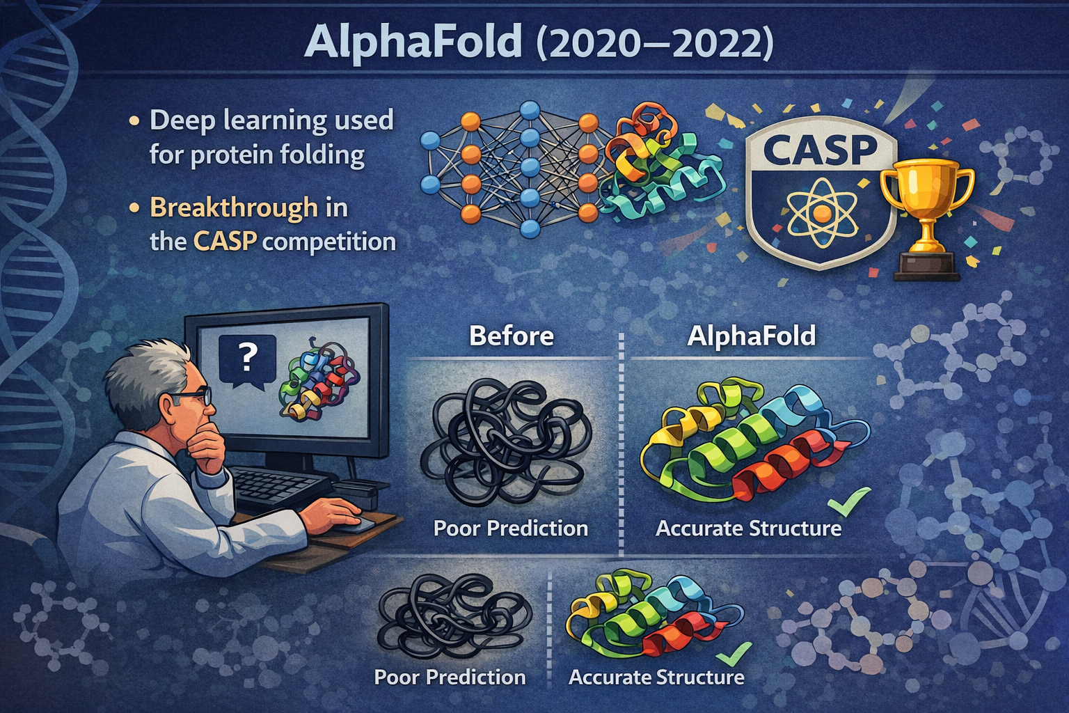
AI progress often occurs through algorithmic breakthroughs, enabling machines to outperform humans in increasingly complex tasks.

Recent studies suggest that AI creates a “jagged frontier.” (Dell’Acqua et al. 2023), i.e., some tasks are well suited to AI, while others that appear similar remain outside its capabilities.

• Within this frontier, AI can strongly enhance knowledge work, improving productivity and the quality of outputs.
• Outside the frontier, AI can reduce performance, especially when users rely too heavily on its outputs without verification.

Figure based on the work of Hendrycks et al. (2025) on Artificial General Intelligence.

Architecture

Evolution of data architectures

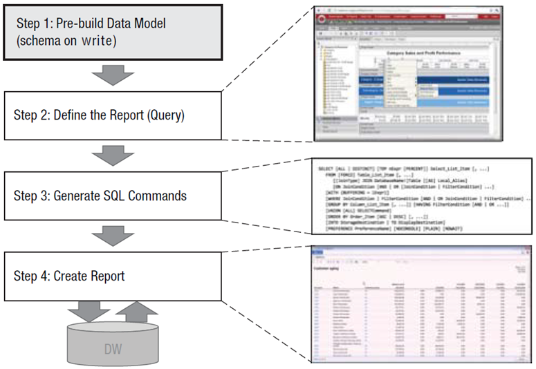
Data architectures have evolved as organizations seek to support more diverse data and increasingly advanced analytics.

Data warehouse

• Integrated, structured data
• High quality and consistency
• Reporting and BI
• Focus: single source of truth

Data lake / lakehouse

• Structured + unstructured data
• Raw data retained at scale
• Supports exploration and ML
• Focus: flexibility

Federated architectures

• Data remains across domains
• Shared access and standards
• Data products / data mesh
• Focus: distributed ownership

AI-ready architecture

• Data + models + AI services
• Real-time and unstructured data
• ML pipelines, vectors, RAG
• Focus: operationalizing AI

➡ Architectural evolution reflects changing business trade-offs:
consistency → flexibility → decentralization → AI integration

Analytics processes

Maturing analytical capabilities

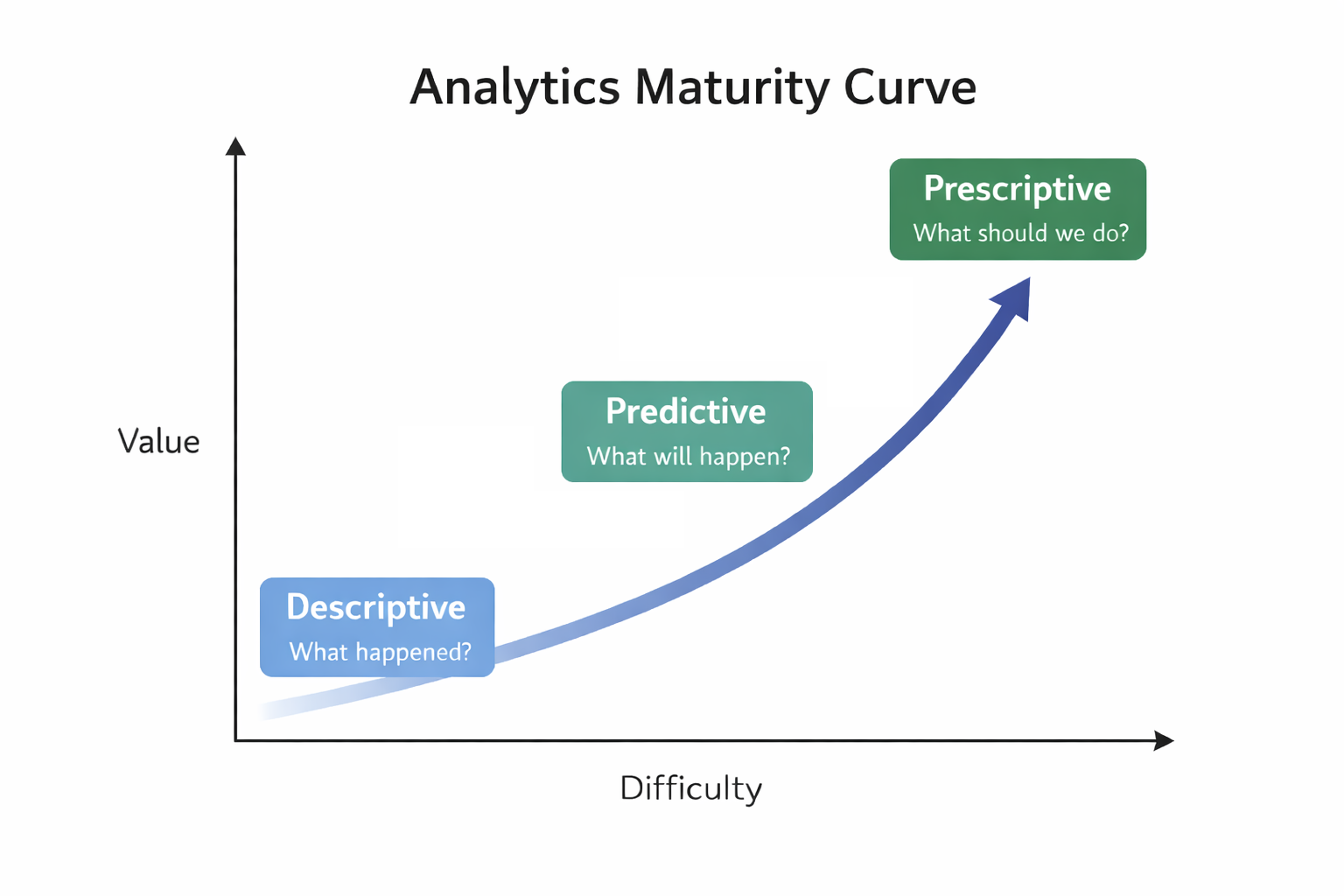
Descriptive analytics: What happened?

• Summarizes historical data to understand patterns and trends.
  
• Example: Sales reports, dashboards, KPIs

Predictive analytics: What will happen?

• Uses statistical models and machine learning to forecast future outcomes.
  
• Example: Demand forecasting, churn prediction

Prescriptive analytics: What should we do?

• Recommends actions based on predictions and optimization.
  
• Example: Pricing optimization, recommendation systems

A particular method, such as regression or machine learning, can serve multiple purposes.

Example: Descriptive analytics

Example: Predictive analytics

Example: Prescriptive analytics

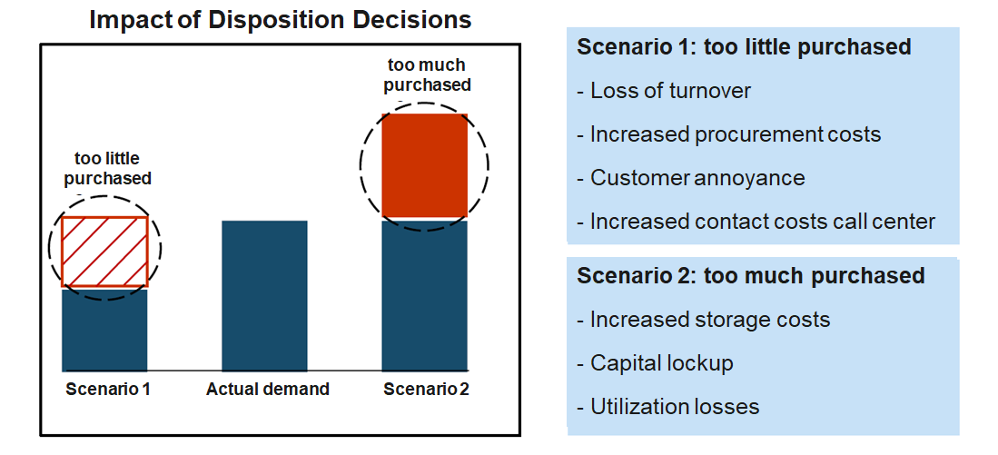
Based on more than 300 million data records per week, Otto generates over one billion forecasts annually on the expected sales of individual products in the coming days and weeks. These forecasts are used to optimize inventory decisions, determining how many units of each product should be stocked or reordered across warehouses. By systematically adjusting inventory levels based on these data-driven recommendations, Otto is able to reduce its overall inventories by up to 30% on average while maintaining product availability.

Source: http://www.bvl.de/misc/filePush.php?mimeType=application/pdf&fullPath=/files/441/442/777/1015/DLK12_C3-3_Praesentation_Stueben.pdf

Exercise: Identify the analytical purpose

Classify each question or statement as descriptive, predictive, or prescriptive analytics.

Business question / statement	Analytical purpose
How many customers cancelled their subscriptions last month?
Which customers are likely to cancel their subscriptions next month?
Offer a 15% discount to customers with a high predicted churn risk.
What were our highest-selling products last quarter?
How much demand should we expect for each product next month?
Reorder 5,000 units to minimize the risk of stock-outs.
Which regions had the highest employee turnover last year?
How many employees are likely to leave during the next 12 months?
Increase recruiting capacity by 20% to maintain required staffing levels.

Cross-Industry Standard Process for Data Mining (CRISP-DM)

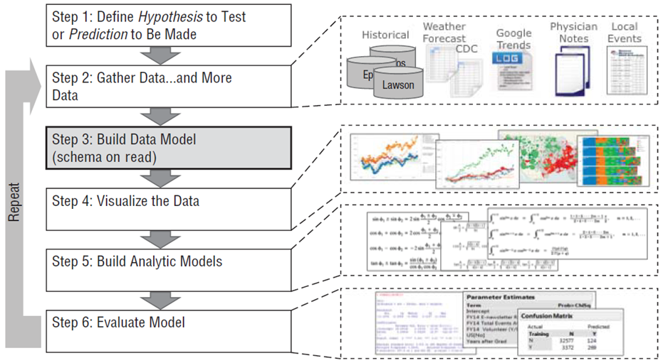
CRISP-DM is a widely used framework that structures data mining and analytics projects (Wirth and Hipp 2000).

• Developed by an industry consortium (e.g., DaimlerChrysler, SPSS, NCR) to create a common methodology for data mining projects.
• Designed to be independent of specific industries and technologies, making it applicable across many domains.
• Integrates best practices from real-world projects, helping teams plan, communicate, and document analytics work.
• Became popular because it provides a reliable and repeatable standard process for managing complex data mining projects.

Alternative models include the Data Science in R workflow, the KDD Process, SEMMA, or TDSP.

Data preparation

Foundations

Before building analytical models, analysts typically engage in data preparation and exploratory data analysis (EDA).

These activities are closely intertwined and often iterative: we prepare and structure the data while simultaneously exploring it to understand its characteristics and potential issues.

Typical activities include:

• Data preparation (e.g., structuring, cleansing, integration)
• Descriptive statistics (e.g., mean, variance, frequencies)
• Visualization techniques (e.g., histograms, boxplots, scatterplots)

Goal: develop an initial understanding of the data, detect patterns or anomalies, and ensure that the data is suitable for further analysis or modeling.

Data types

Conducting EDA and representing the “real world” requires us to use appropriate data types. Typically, we distinguish four fundamental data types, known as measurement scales:

Qualitative description of objects

• Nominal (special case: binary)
• Ordinal

Quantitative description objects

• Interval
• Ratio

Qualitative: Nominal scale

• Values of a nominal (aka. categorical) attribute are symbols or names of things
• Each value represents some kind of category, code, or state.
• This scale assumes existence of a finite number of equivalency classes, where each class is named or labeled.
• The values do not have any meaningful order.

Examples:

• Hair color = {black, blond, brown, gray, red, white, …}
• Postal codes = {96047, 96048, …}

Special case of the nominal scale: Binary scale – also called Boolean

• Nominal attribute with only 2 states
• 0/FALSE typically means absence and 1/TRUE presence.

Examples:

• Smoking: 1 indicates patients in a trial that smoke, 0 otherwise.
• Purchase: 1 indicates that a person purchased a product, 0 otherwise.

Qualitative: Ordinal scale¹

• A categorical attribute with values that have a meaningful order, but the magnitude between successive values is not known
• The ordinal scale is useful for registering subjective assessments and things that cannot be measured objectively (often used in surveys for ratings)

Values cannot be multiplied or added, even if the numbers belong to the same scale.

Relations between values:

• Transitivity: If A>B, B>C, then A>C,
• Symmetry: : If A>B, then B<A

Examples:

• School grades = {A < B < C < D < E < F} or {1 < 2 < 3 < 4 < 5 < 6}
• Places in a competition = {1st, 2nd, 3rd, 4th, …}

1. Also known as a “rank scale”.

Quantitative: Interval scale

• A numeric measurable attribute in the form of integer or real values. The distance between the numbers or units on this scale is equal over all levels of the scale. Values of the interval scale have no natural “zero” point.
• Invariant under a linear transformation \(ax + b\), \(a > 0\), \(b \geq 0\)
• Although the sum of two interval-scale measurements is not meaningful by itself, their average can be computed

Examples:

• Celsius scale of temperature (there is no natural zero, 0°C is arbitrarily defined), a Celsius value \(c\) can be linearly transformed to a Fahrenheit value \(f\): \(f = \frac{9}{5}c + 32\)
• Dates and time (e.g., conversion from Julian to Gregorian calendar is possible)

Quantitative: Ratio scale

• Numeric values with a meaningful zero point (e.g., “zero” means absence)
• All arithmetic rules and functions can be applied (addition, subtraction)

Examples:

• Money, person’s age, market share, quantities purchased, speed, …
• Kelvin (K) temperature, which has a true zero-point (\(0\,K = -273.15\,^\circ C\)): It is the point at which the particles that comprise matter have zero kinetic energy

Scales and mathematical operations

Due to the different mathematical properties, not all statistical measures can be computed on different measurement scales:

Scale	Mathematical operations possible	Mode	Frequency	Percentiles / Median	Mean / Variance / SD
Nominal	\(=, \neq\)	X	X
Ordinal	\(=, \neq, <, >\)	X	X	X
Interval	\(=, \neq, <, >\), linear transformation	X	(X)	X	X
Ratio	\(=, \neq, <, >, \times, /, +, -\)	X	(X)	X	X

(X) The frequency (relative / absolute) may be calculated for a numeric variable, but makes only sense when the number of possible values is low

Data quality and preparation

In business analytics, we rarely work with carefully curated datasets. Instead, data often comes from multiple systems, processes, and teams, where it is primarily created for operational purposes rather than analysis. Because these data sources are not always standardized or under the analyst’s control, quality issues are common:

• Missing values (e.g., incomplete historical market data)
• Outdated values (e.g., customer address has changed)
• Inconsistent formats or units (e.g., dates stored as text, mixed currencies)
• Duplicate records (e.g., customers with multiple accounts)
• Measurement or data entry errors (e.g., human data entry, broken sensors)

Before conducting analysis, we must ensure that the data is fit for use (Strong et al. 1997).

Typical data preparation actions

1. Data structuring
2. Data cleansing
3. Data integration
4. Data transformation

In many real-world analytics projects, data preparation and cleaning can take up to ~80% of the total effort.

Data structuring: Example

There are many ways to structure the same dataset.

Option A (wide)

Region	Year	Sales_Q1	Sales_Q2	Sales_Q3	Sales_Q4
Europe	2023	120	140	160	150
Asia	2023	100	110	120	130

Option B (long)

Region	Year	Quarter	Sales
Europe	2023	Q1	120
Europe	2023	Q2	140
Europe	2023	Q3	160
Europe	2023	Q4	150
Asia	2023	Q1	100
Asia	2023	Q2	110
Asia	2023	Q3	120
Asia	2023	Q4	130

➡ Which would you select as an input for a data analytics tool?

→ Solution: Option B, because this is what data analytics tools typically expect.

Data structuring: Principles

Data structure typically expected by data analytics tools

Vocabulary

• A dataset is a collection of values (e.g., nominal, categorical, numeric).
• Each value belongs to a variable and an observation

Expected data structure

• Each variable forms a column
• Each observation forms a row
• Each type of observational unit forms a table

Data must be structured according to the expectations of the analytical tool being used. Reviewing the tool’s documentation and example datasets can help clarify the required format.

Based on the Tidyverse and the work of Wickham (2014).

Data structuring: Example continued

Dataset df (wide)

Region	Year	Sales_Q1	Sales_Q2	Sales_Q3	Sales_Q4
Europe	2023	120	140	160	150
Asia	2023	100	110	120	130

Convert wide → long

long_df <- df |>
  pivot_longer(
    cols = starts_with("Sales_"),
    names_to = "Quarter",
    values_to = "Sales"
  )

long_df

Result:

Region	Year	Quarter	Sales
Europe	2023	Sales_Q1	120
Asia	2023	Sales_Q1	100
Europe	2023	Sales_Q2	140
Asia	2023	Sales_Q2	110
…	…	…	…

Data structuring: Example continued

As a last step, we need to clean the Quarter column by removing the "Sales_" prefix:

long_df <- long_df |>
  mutate(Quarter = str_remove(Quarter, "^Sales_"))

Final tidy dataset:

Region	Year	Quarter	Sales
Europe	2023	Q1	120
Europe	2023	Q2	140
Europe	2023	Q3	160
Europe	2023	Q4	150
Asia	2023	Q1	100
Asia	2023	Q2	110
Asia	2023	Q3	120
Asia	2023	Q4	130

Note: we will cover selected transformation operations like melt in the exercises.

Data cleansing

Data issue	Example	Data cleansing action
Missing values	Historical market data missing for some days	Impute values (e.g., interpolate prices), fill with mean/median, or mark as NA
Outdated values	Customer moved but old address still stored	Update records from CRM, external address verification service
Outliers / implausible values	Age = 250, salary = −5000	Detect and remove, cap values, or replace with plausible values
Inconsistent formats	Dates stored as "03/01/23" and "2023-01-03"	Standardize to a single format (e.g., ISO date YYYY-MM-DD)
Inconsistent units	Revenue in USD and EUR mixed in one column	Convert to common currency
Duplicate records	Same customer registered twice	Identify duplicates and merge records
Data entry errors	"Munich" vs "Munch"	Correct spelling using reference tables
Sensor errors	Temperature sensor reports 9999	Remove invalid values or replace with interpolated measurements

Data integration

Organizations often store data in different systems (e.g., CRM, sales systems, web analytics).

Customer database (CRM)

Customer_ID	Name	Country	Email
101	Alice	Germany	alice@example.com
102	Bob	France	bob@example.com
103	Clara	Germany	clara@example.com

Sales transactions

Customer_ID	Order_ID	Revenue
101	5001	200
101	5002	150
103	5003	300

For analysis, we can integrate these datasets using the shared key Customer_ID.

integrated_data <- customers |>
  inner_join(sales, by = "Customer_ID")

This creates a combined dataset that links customer information with sales.

Customer_ID	Name	Country	Email	Order_ID	Revenue
101	Alice	Germany	alice@example.com	5001	200
101	Alice	Germany	alice@example.com	5002	150
103	Clara	Germany	clara@example.com	5003	300

For analytical purposes, redundant values are often acceptable. The goal is to organize data into a tidy structure, where each row represents one observation and all relevant variables are available for analysis.

Data transformation: Example

Often, the way data is stored determines which mathematical operations are possible.

Example: timestamps stored as strings

user_id	timestamp
101	“2025-03-12 14:23:05”
102	“2025-03-12 18:02:11”
103	“2025-03-13 09:15:42”

If treated as a string, we can only perform operations such as:

• equality checks (\(=\) / \(\neq\))
• simple filtering or sorting

This severely limits analysis.

Format conversions help transform raw data into representations suitable for EDA and analytical models:

Representation	Example	Possible analysis
Numeric timestamp	1741789385	time differences, time series
Hour of day	14	activity patterns during the day
Day of week	Wednesday	weekday vs. weekend behavior
Day of year	71	seasonal patterns

Data preparation transforms raw data into formats that allow meaningful mathematical operations and analysis.

Summary

• Modern machine learning and AI for big data were enabled by more computing power, new algorithms, new architectures, and new analytics processes.
• Analytics capabilities have developed from descriptive toward predictive and prescriptive purposes.
• CRISP-DM structures analytics as an iterative process connecting business understanding, data, modeling, and evaluation.
• Data preparation structures, cleans, integrates, and transforms raw data into tidy analytical data.

Feedback

Please take 1–2 minutes to reflect on today's session.

Complete the short feedback survey

References

Dell’Acqua, Fabrizio, Edward McFowland, Ethan Mollick, et al. 2023. Navigating the Jagged Technological Frontier: Field Experimental Evidence of the Effects of AI on Knowledge Worker Productivity and Quality. Working Paper Nos. 24-013. Harvard Business School.

Hendrycks, Dan, Dawn Song, Christian Szegedy, et al. 2025. “A Definition of AGI.” In arXiv Preprint arXiv:2510.18212.

Strong, Diane M, Yang W Lee, and Richard Y Wang. 1997. “Data Quality in Context.” Communications of the ACM 40 (5): 103–10. https://doi.org/10.1145/253769.253804.

Wickham, Hadley. 2014. “Tidy Data.” Journal of Statistical Software 59: 1–23.

Wirth, Rüdiger, and Jochen Hipp. 2000. “CRISP-DM: Towards a Standard Process Model for Data Mining.” Proceedings of the 4th International Conference on the Practical Applications of Knowledge Discovery and Data Mining 1: 29–39.