Analytics & Big Data

Session 9: Big data 2

Prof. Dr. Gerit Wagner

(2026-05-04)

• Explain and interpret the core ideas and mathematical operations underlying artificial neural networks
• Distinguish between major neural network architectures (MLP, CNN, RNN, TM) and identify the types of data for which they are most appropriate.
• Understand the design and training process of neural networks, including architecture selection and optimization.

Foundations

From biological neurons to artificial neural networks

Key milestones

• 1943 (Warren McCulloch & Walter Pitts) — Mathematical model of artificial neurons
• 1958 (Frank Rosenblatt) — Development of the Perceptron
• 2010s (Geoffrey Hinton, Yann LeCun & Yoshua Bengio) — Revival of modern deep learning
• 2020s (GPT models, OpenAI) — Emergence and widespread adoption of large language models (LLMs) and multimodal AI systems

Highlight: multimodal AI (big-data) is closely connected to neural networks

Inputs correspond to dendrites, outputs to axons

The foundations of neural networks were developed 80 years ago. Why did we have to wait for the AI breakthroughs for so long?

-> AI-Winters: 1974-1980, 1987-1993

-> availability of computing power and data (next slide)

Performance of machine learning and neural networks

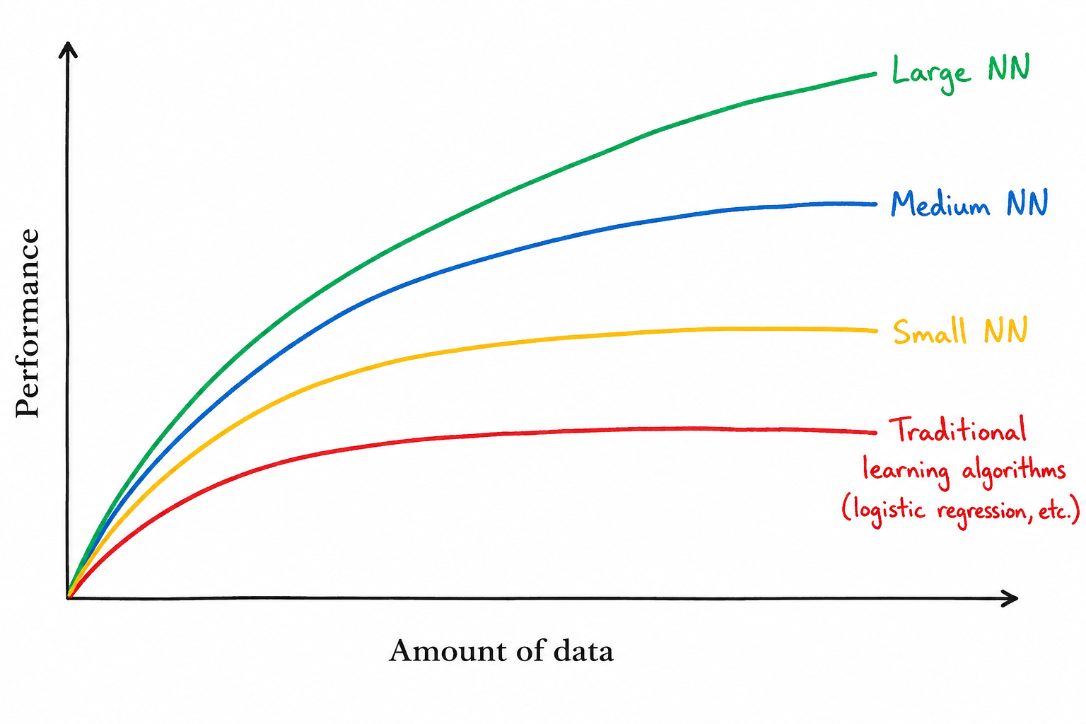
Key drivers of recent progress in neural networks

• Availability of large-scale datasets

• Increasing computational power (especially GPUs/TPUs)

• Advances in algorithms and neural network architectures

• Specialization of neural networks:

  • Convolutional Neural Networks (CNNs) for image and video recognition
  • Recurrent Neural Networks (RNNs) for sequential and time-series data
  • Transformers for language processing and generative AI
  • Graph Neural Networks (GNNs) for network and relational data
  • Diffusion Models for image and media generation

TPU: Tensor processing unit (for matrix and tensor operations in AI)

In small-data regimes, experiments are needed to identify algorithms that perform best for a given dataset.

The perceptron

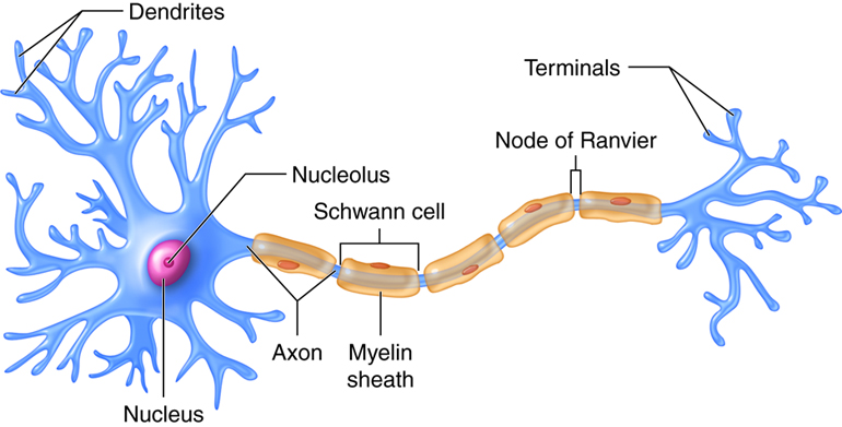
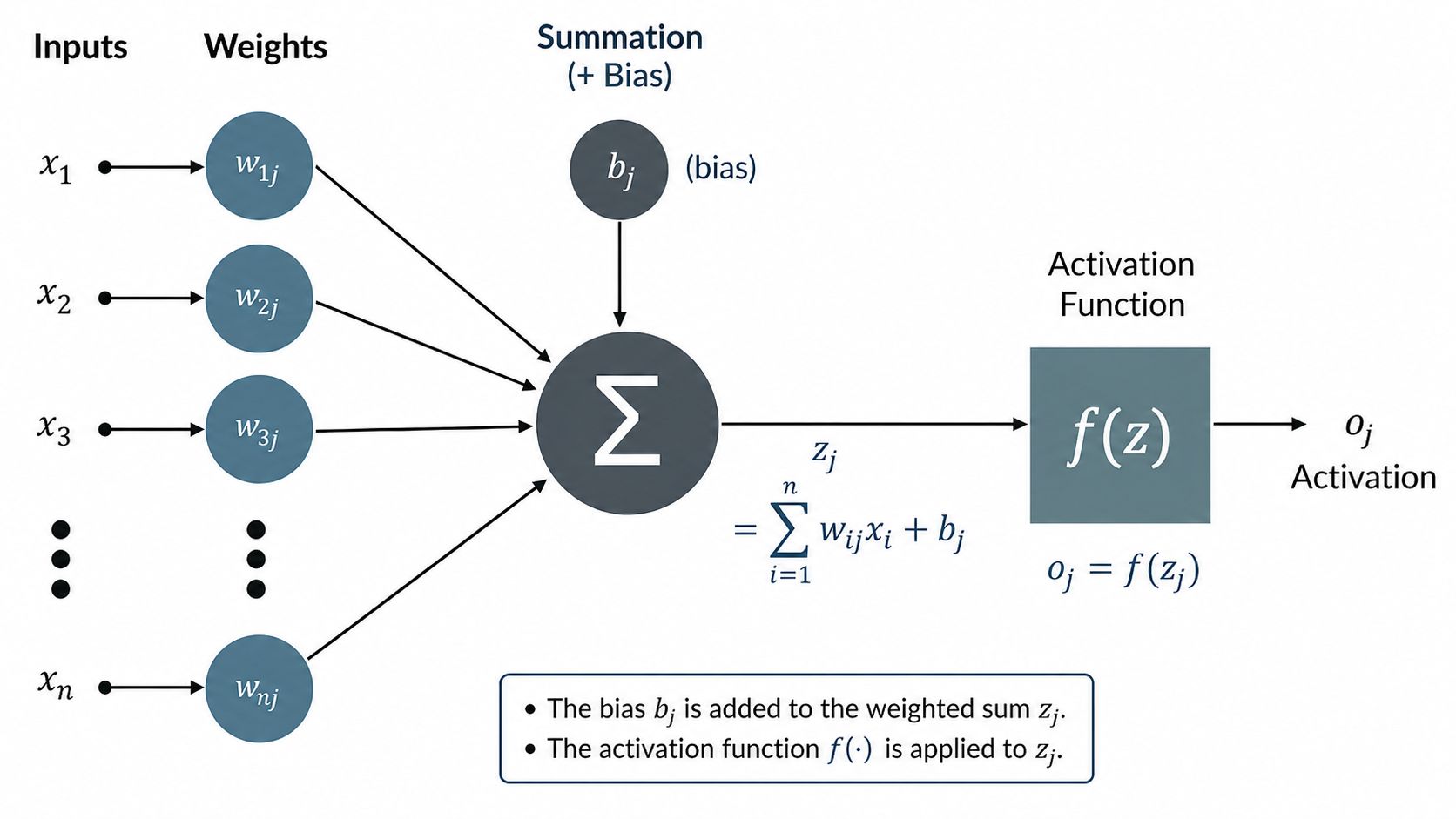
A perceptron is one of the earliest forms of neural networks. A classical perceptron is characterized by:

\[z = w^T x + b\]

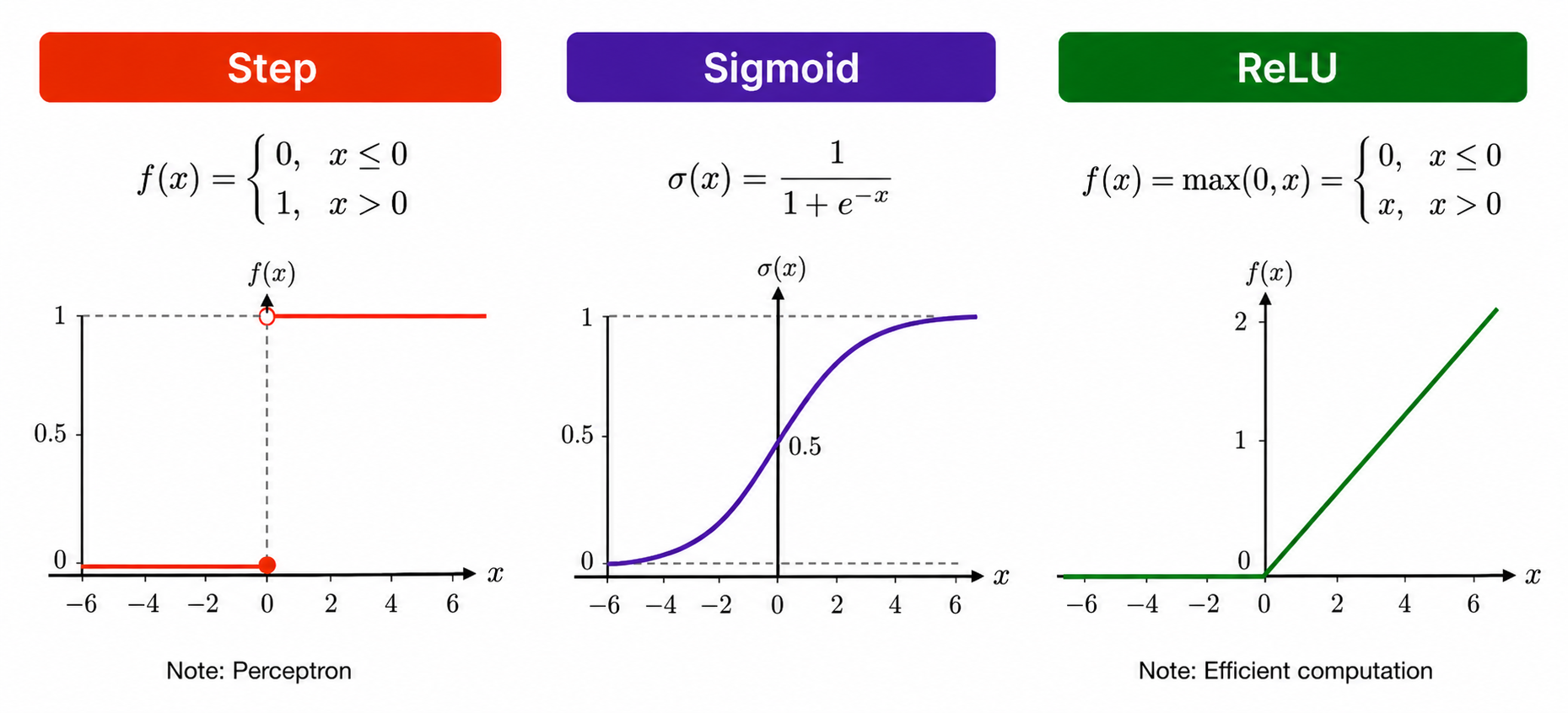
followed by a threshold activation:

\[\hat{y} = \begin{cases} 1 & \text{if } w^T x + b > 0 \\ 0 & \text{otherwise} \end{cases}\]

• This corresponds to a linear classifier
• The training of the perceptron consists of feeding it multiple training samples and calculating the output for each of them
• After each sample, the weights \(w\) are adjusted to minimize a loss function, which quantifies the difference between the predicted and true outputs

From perceptron to deep neural networks

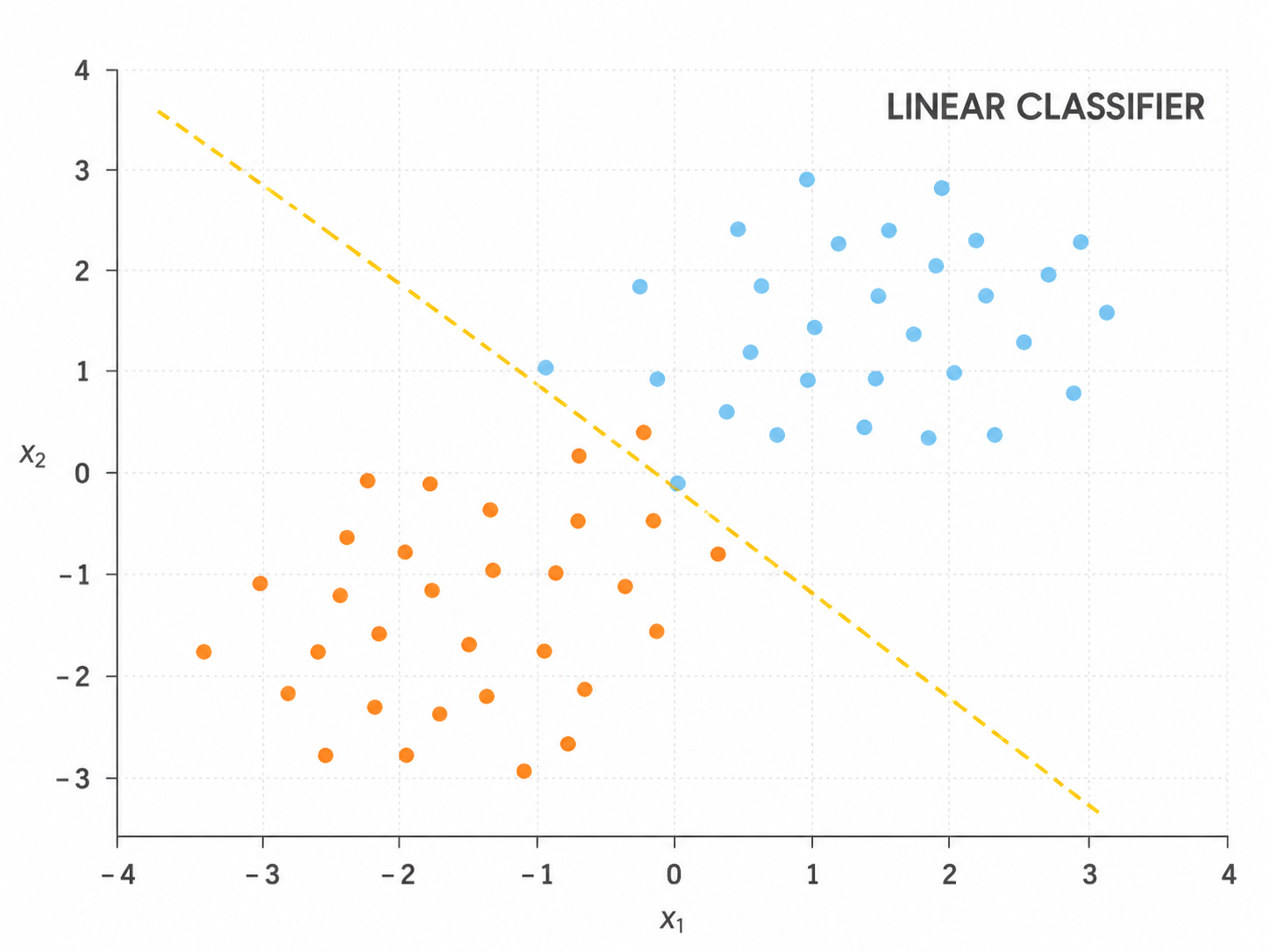
Limitation of a single perceptron: It cannot build abstract intermediate representations and can only learn linear decision boundaries.

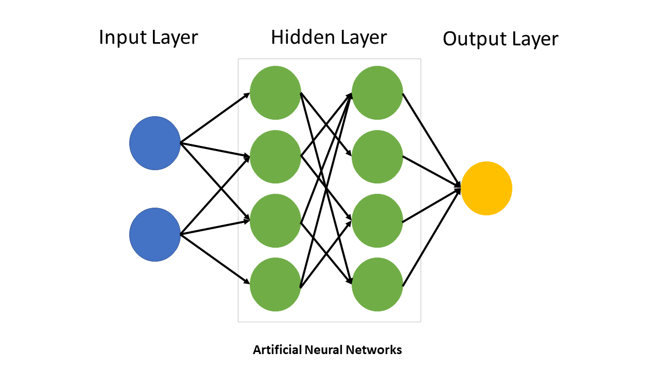
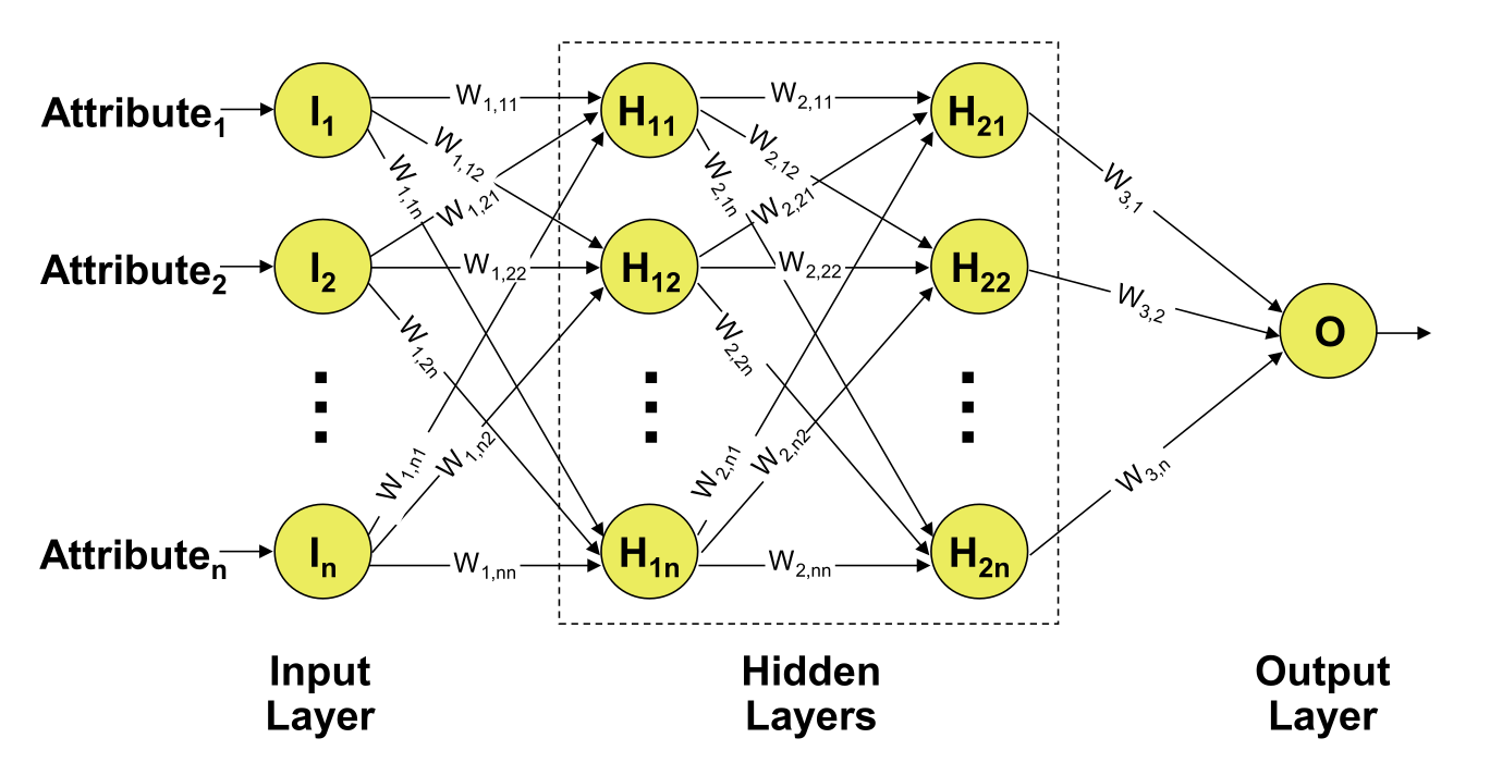
Solution: Multilayer neural networks combine:

• Multiple hidden layers, which enable increasingly abstract representations
• Activation functions, which make nonlinear learning possible

Layers:

• Input neurons: raw data (e.g., images, audio, video)
• Hidden neurons: the weights and biases store abstract representations learned from the data (e.g., edges, parts of an image)
• Output neuron: prediction (e.g., one neuron for binary, multiple for multi-class)

Note: the number of layers and neurons is specified ex-ante and does not change in the training process.

🎥 Grant Anderson (3Blue1Brown) provides a series of instructive
animated explanations, including one on Neural Networks.

Functionality of a neuron

In a classical perceptron, the activation is typically binary (0 or 1), representing whether the neuron “fires.”
In modern neural networks, activations are usually continuous-valued scalars determined by the activation function.

Types of activation functions

Advantage of Sigmoid activation: smooth, supports gradient descent Note: in the case of Sigmoid activation, the NN is basically a network of logistic regressions ReLU: for efficient computation

ReLU: Rectified Linear Unit.

Training of a multilayer perceptron

• Weights are initialized with carefully selected random values
• For each training item, the predicted output is calculated (“forward pass”)

Loss function

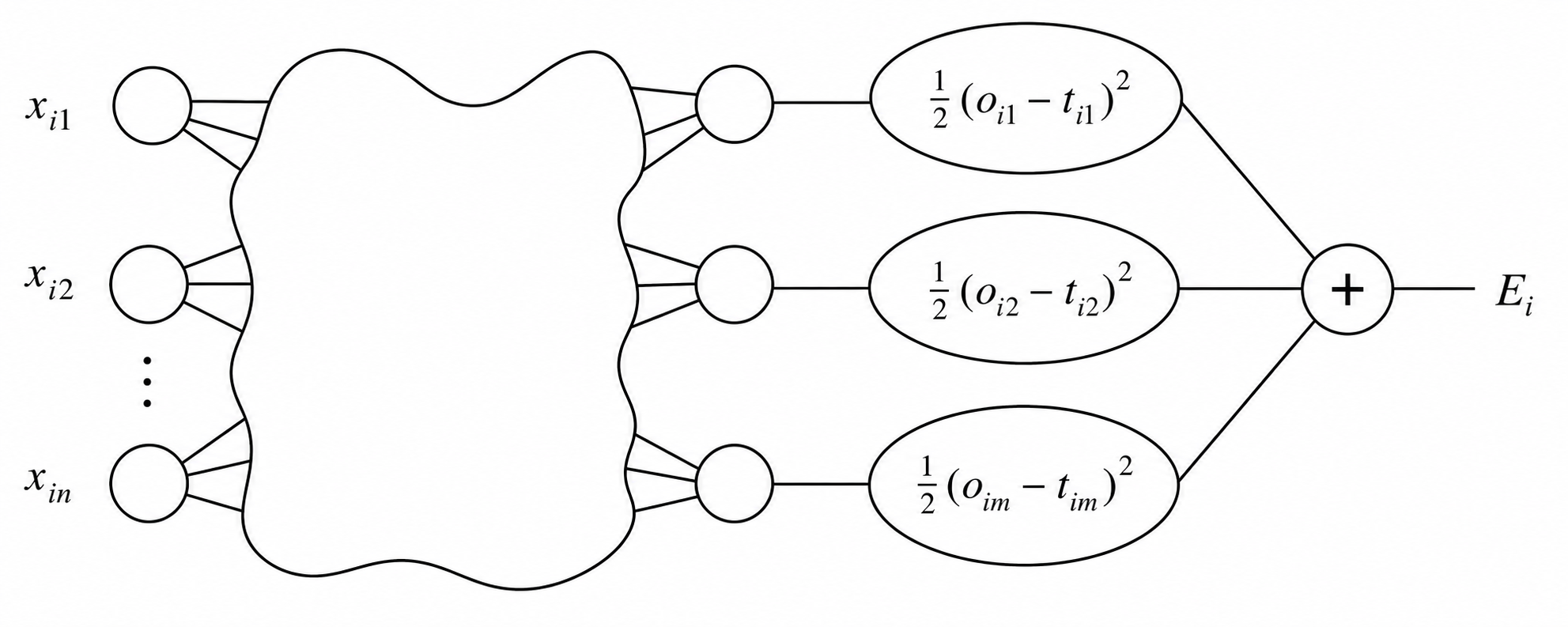
The network’s prediction error is measured with a loss function.

For one training example \(i\):

\[E_i = \frac{1}{2} \sum_{j=1}^{m} (o_{ij} - t_{ij})^2\]

This is the squared error loss across all output neurons \(j\).

Across all \(h\) training examples, the total loss is:

\[E = \sum_{i=1}^{h} E_i\]

Backpropagation adjusts the weights to reduce this total loss.

The \(1/2\) makes the math cleaner for the derivatives.

Backpropagation

Backpropagation calculates the gradients of the loss function with respect to the network’s weights. These gradients are then used by an optimizer, to iteratively update the weights and reduce the difference between predicted and true outputs.

initialize weights and biases

repeat until stopping criterion is met:

    total_error = 0

    for each training example:

        pass input forward through all layers
        compare predicted output with target value
        add error to total_error
        propagate error backward through all layers
        update weights and biases

    check whether total_error is small enough

Using the loss function to adjust weights

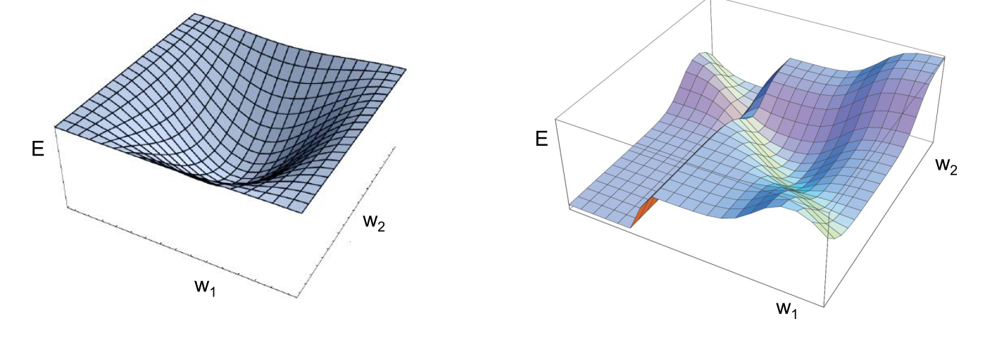
The loss function \(E\) has to be minimized. Because it depends on the output neurons \(o_j\), it automatically depends on their weights to the precedent layer(s):

\[o_j=f(s(x)_j) \text{ with } s(x)_j =\sum_k^n w_{jk}\cdot x_k\]

Thus, the weights have to be found where \(E\) is minimal.

Examples of the loss function with two weights (simplified):

Gradient descent

To minimize the loss function \(E\) the backpropagation algorithm uses the method of gradient descent. This method searches those weights, where the vector containing the partial first derivatives of the loss function \(\nabla E\) (gradient) is equal to the zero vector (minimum):

\[ \nabla E = \left( \frac{\partial E}{\partial w_1}, \frac{\partial E}{\partial w_2}, \ldots, \frac{\partial E}{\partial w_m} \right) \]

To adjust the weight \(w_{ij}\), which connects neuron \(i\) to neuron \(j\), gradient descent updates the weight in the negative gradient direction:

\[ \Delta w_{ij} = -a \cdot \frac{\partial E}{\partial w_{ij}} \]

\[ \Delta w_{ij} = -a \cdot \sum_{j=1}^{m} (o_{ij} - t_{ij}) \cdot (-x_i) = a \cdot \sum_{j=1}^{m} (o_{ij} - t_{ij}) \cdot x_i \]

where \(a\) represents the predefined learning rate. The adjusted weight is then computed as:

\[ w_{ij}^{\text{new}} = w_{ij}^{\text{old}} + \Delta w_{ij} \]

Because neural networks have many parameters, each update changes the model in many dimensions at once. The learning rate therefore has to be chosen carefully: large steps can destabilize training, while very small steps can make learning inefficient.

Specialized NNs

Overview

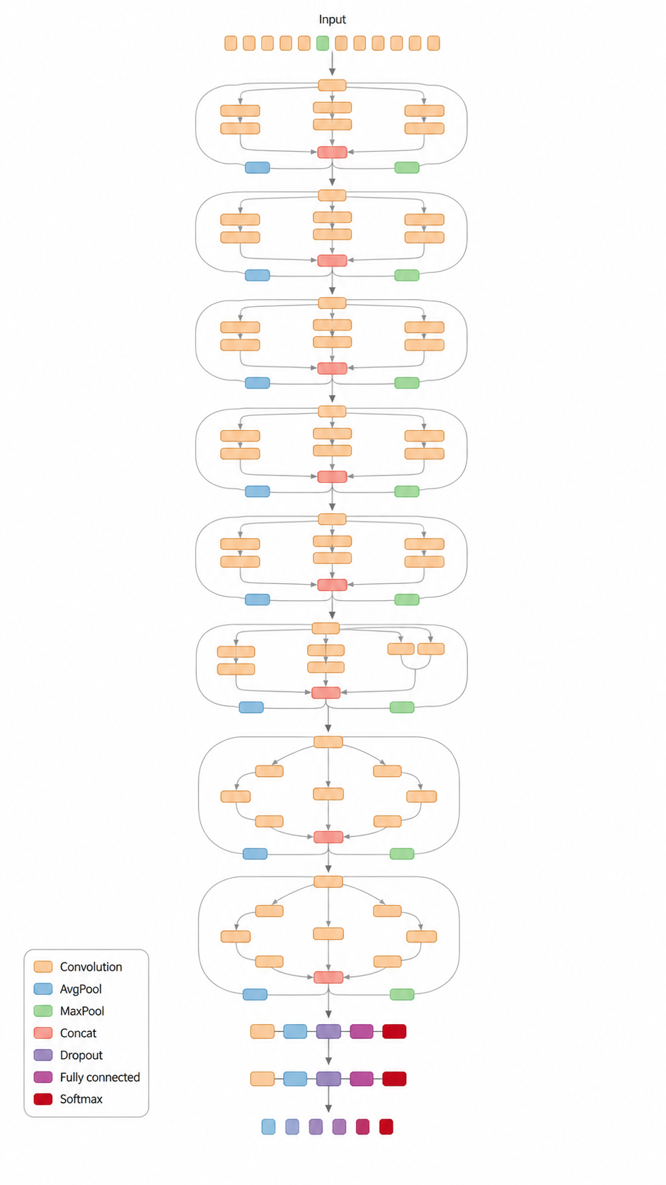
Basic neural networks are often introduced as fully connected feed-forward networks. Specialized architectures go beyond this and differ in the following design choices:

Design choice	How architectures differ
Input structure assumed	Different architectures are built for different data structures, such as tabular data (MLPs), spatial data and images (CNNs), sequence data (RNNs or Transformers), relational data (graph neural networks), or ; generative tasks (GANs).
Neuron / unit type	The basic unit may be a dense neuron, recurrent cell, gated LSTM/GRU cell, attention head, or a generator/discriminator module.
Layer operation	Layers may perform matrix multiplication, convolution with moving filters, recurrent state updates, self-attention, or adversarial generator/discriminator training.
Connectivity pattern	Information may flow through all-to-all dense connections, local sliding windows, temporal loops with hidden states, or token-to-token attention.

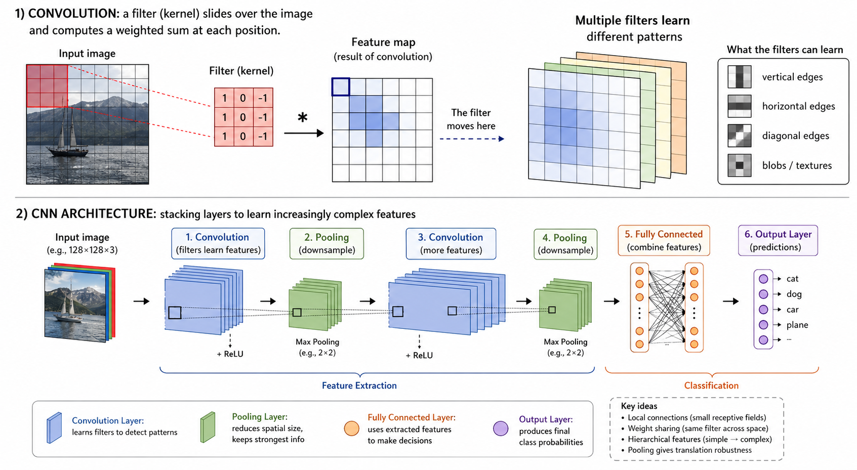
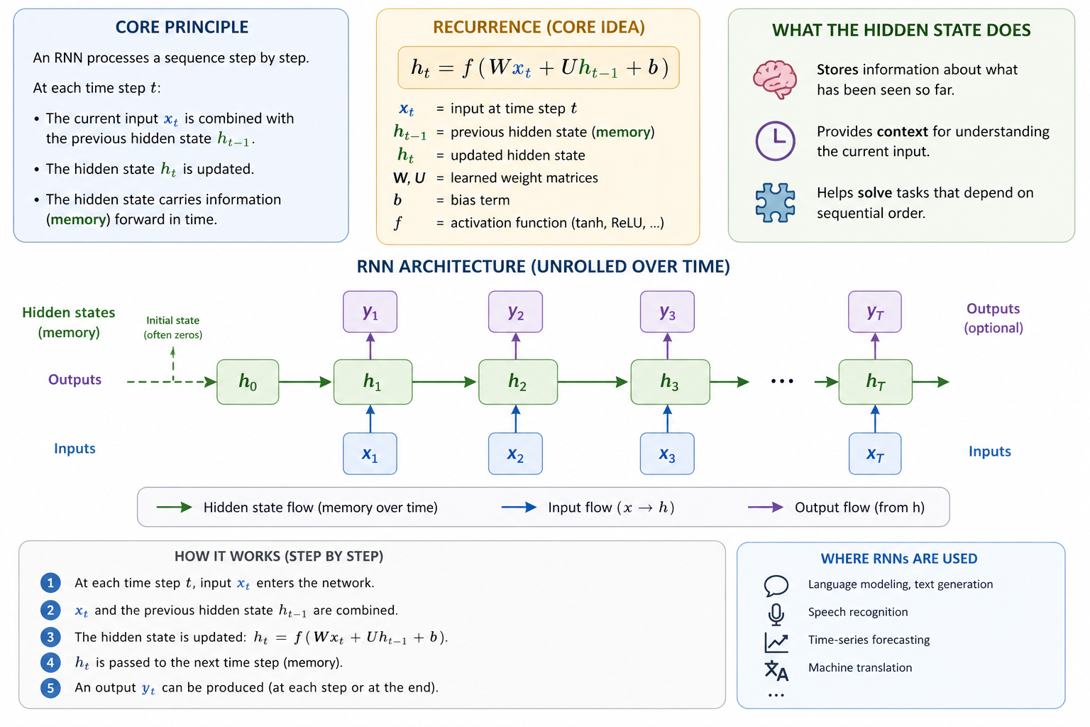
Focus in this section: We use CNNs, RNNs, and Transformers as key examples because they show three central architectural ideas:

• Convolution through moving filters
• Memory through recurrence, and
• Attention.

Example architecture: Inception-ResNet-v2

This slide should not present CNNs, RNNs, and Transformers as three isolated summaries. The teaching point is that specialized neural networks encode assumptions about data structure. CNNs reuse local filters over spatial data; RNNs reuse recurrent cells over time; Transformers compare tokens through attention. GANs are useful as an additional example because their specialization is not mainly a layer type, but a training setup with two networks: generator and discriminator.

Inception-ResNet-v2: coders basically build DAGs in code and generate the architecture charts as an overview.

Convolutional neural networks (CNN)

Convolution layers: effectively multiply the number of input neurons, e.g., a 28x28x1 grayscale image with 32 filters leads to 28x28x32=25,088 activations.

TBD: similar to SVM: kernels facilitate learning in higher-dimensional transformations.

Recurrent neural networks (RNN)

Transformers

Design and training of neural networks

Modeling: choose the architecture and training setup

Best-practice logic Start with choices that are mostly determined by the data structure and the prediction task.
Then tune the parts that require experimentation.

Architecture family

Data structure	Typical model	Inductive bias
📊 Tabular data	MLP	fully connected
📷 Images	CNN	local / spatial
🎧 Audio	CNN / RNN / Transformer	local, sequential, attention
⏱️ Time series	RNN / Transformer	temporal order
📝 Text / language	Transformer	global attention

Output layer and loss function

Prediction task	Output layer	Output activation	Loss function
Regression	1 neuron	Linear	MSE
Binary classification	1 neuron	Sigmoid	Binary cross-entropy
Multi-class classification	One neuron per class	Softmax	Categorical cross-entropy

Rule of thumb: data structure determines the architecture; prediction task determines the output layer and loss.

Training setup choices

Besides the selection of the model type, output layer, and loss function (see previous slide), these choices are usually standardized:

• Adam is a strong default optimizer
• Hidden layers usually start with ReLU

These choices require more experimentation to tune complexity and parameters:

1. Network structure
   How much can the model represent?

Depth
number of layers

• shallow → simple patterns
• deep → complex abstractions

Width
neurons per layer

Typical starts:
32, 64, 128, 256

2. Learning rate \(\eta\)
   How large are the update steps?

\[ w := w - \eta \nabla_w J \]

• too high → unstable
• too low → slow

Typical range:
\(10^{-3}\) to \(10^{-4}\)

3. Regularization
   How do we reduce overfitting?

• Dropout
  randomly disables units
• Weight decay
  penalizes large weights
• Early stopping
  stops before overfitting
  
  
  
  

Optimizer: updates weights (similar to \(w^{new} = w^{old} - a \cdot \frac{\partial E}{\partial w}\), but more advanced: using information from previous gradients).

Note: Neural networks and feature engineering

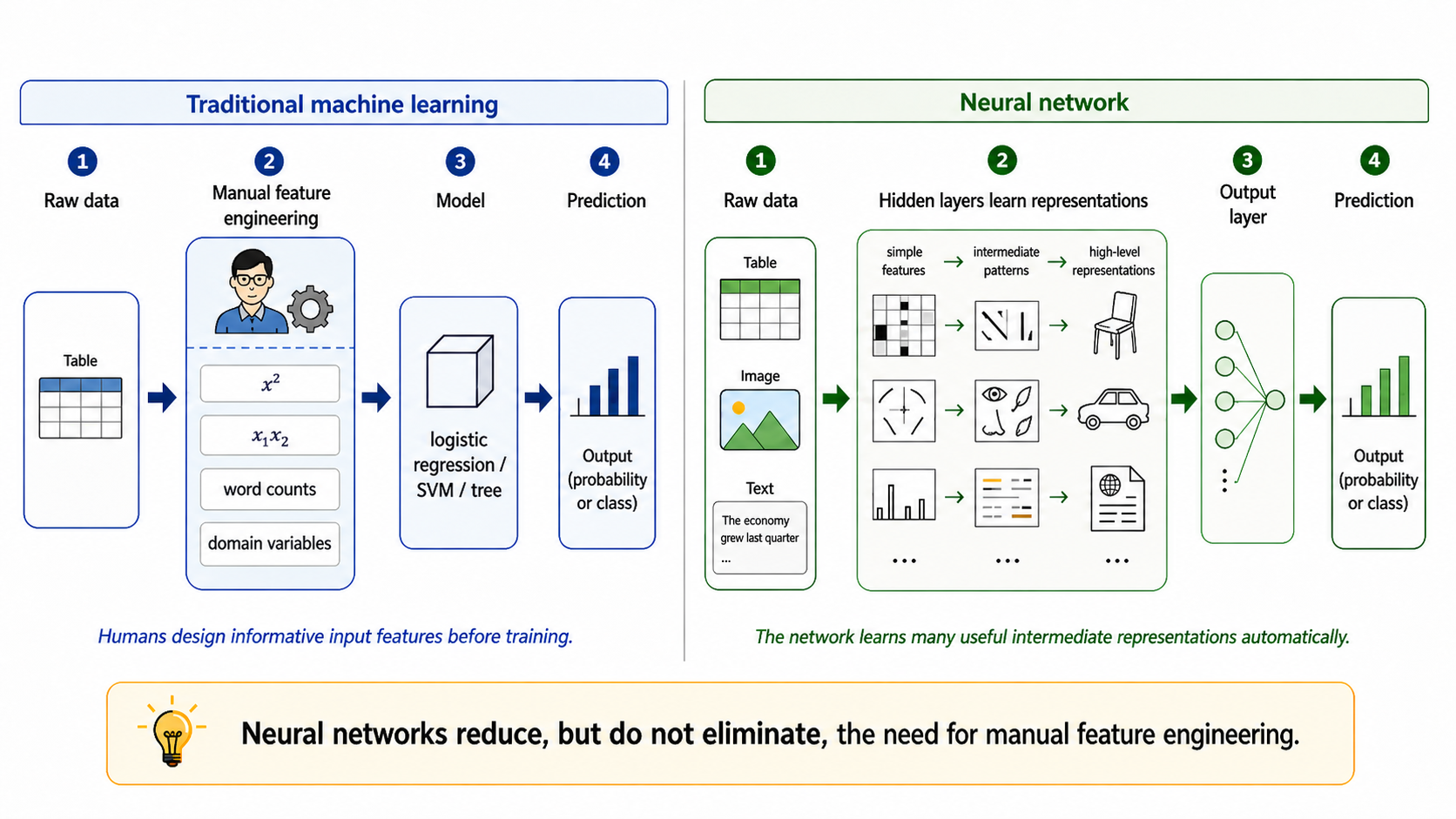
Traditional machine learning often relies strongly on manual feature engineering: humans design useful input variables before training the model. Neural networks can reduce this need because hidden layers learn intermediate representations from data. However, feature engineering does not disappear. We still need to decide:

• which data are provided as input
• how inputs are encoded and normalized
• whether domain-specific variables or transformations are added

Python code example

The sklearn library provides basic feedforward networks, including MLPClassifier and MLPRegressor. It does not offer CNNs, RNNs, or other advanced neural networks.

from sklearn.neural_network import MLPClassifier
from sklearn.datasets import make_classification
from sklearn.model_selection import train_test_split

X_train, X_test, y_train, y_test = train_test_split(X, y)

model = MLPClassifier(
    hidden_layer_sizes=(32, 16),  # architecture (depth + width)
    activation="relu",            # hidden activation
    solver="adam",                # optimizer
    learning_rate_init=0.001,     # learning rate
    alpha=0.0001,                 # L2 regularization (weight decay)
    max_iter=200
)
model.fit(X_train, y_train)

PyTorch (I)

For advanced neural networks and production environments, pytorch and tensorflow are suitable libraries.

import torch

X = torch.randn(100, 10)
y = torch.sum(X, dim=1, keepdim=True)  # simple target

# TODO: specify MLP

model = MLP(
    input_dim=10,
    hidden_layers=[32, 16],   # try: [8], [64, 64], [128, 64, 32]
    output_dim=1              # regression
)

# Training setup
criterion = nn.MSELoss()   # regression
learning_rate = 1e-3       # try: 1e-1, 1e-4
optimizer = torch.optim.Adam(model.parameters(), lr=learning_rate)

# Training loop
for epoch in range(100):

    predictions = model(X)  # Forward pass
    loss = criterion(predictions, y)

    # Backpropagation
    optimizer.zero_grad()
    loss.backward()
    optimizer.step()

    print(f"Epoch {epoch}, Loss: {loss.item():.4f}")

The architecture (whether it is a CNN/RNN/Transformer/… is not specified as a parameter, but implied by the design of layers).

PyTorch (II)

import torch.nn as nn

# Specify MLP
class MLP(nn.Module):
    def __init__(self, input_dim, hidden_layers, output_dim):
        super().__init__()

        layers = []
        prev_dim = input_dim

        # Depth and width
        for h in hidden_layers:
            layers.append(nn.Linear(prev_dim, h))
            layers.append(nn.ReLU())
            prev_dim = h

        layers.append(nn.Linear(prev_dim, output_dim))

        self.model = nn.Sequential(*layers)

    def forward(self, x):
        return self.model(x)

# ...
model = MLP(
    input_dim=10,
    hidden_layers=[32, 16],
    output_dim=1
)

See the torch Module for inherited methods.

Summary

• Neural networks transform inputs into outputs through weighted connections, biases, and activation functions.
  A single perceptron can only learn linear decision boundaries; multilayer networks with nonlinear activations can model more complex patterns.

• Training consists of a forward pass, loss calculation, backpropagation, and parameter updates via an optimizer such as gradient descent or Adam.

• Different neural network architectures encode different assumptions about data:
  MLPs for tabular data, CNNs for spatial data, RNNs for sequences, and Transformers for attention-based language tasks.

• Designing neural networks means choosing the architecture, output layer, loss function, learning rate, optimizer, and regularization strategy, then iteratively evaluating and adjusting these choices.

Survey: Session 9

https://forms.gle/1vsCsqc3SzWfSX1f6

Note: Responses may be analyzed and published in anonymized form.

Please complete the survey before you leave today — thank you 🙏

References

Zhang, A., Lipton, Z. C., Li, M., & Smola, A. J. (2023). Dive into deep learning. Cambridge University Press.