Analytics & Big Data

Session 6: Machine learning 1

Prof. Dr. Gerit Wagner

(2026-04-20)

• Distinguish between supervised and unsupervised machine learning approaches and explain the generalization problem in supervised machine learning.
• Describe the workflow of supervised machine learning, including feature engineering, train–test splitting, model training, cross-validation, and evaluation.
• Connect conceptual machine learning procedures to Python implementations, including preprocessing, model training, and evaluation using scikit-learn. (see exercise)

Foundations

Distinguishing concepts

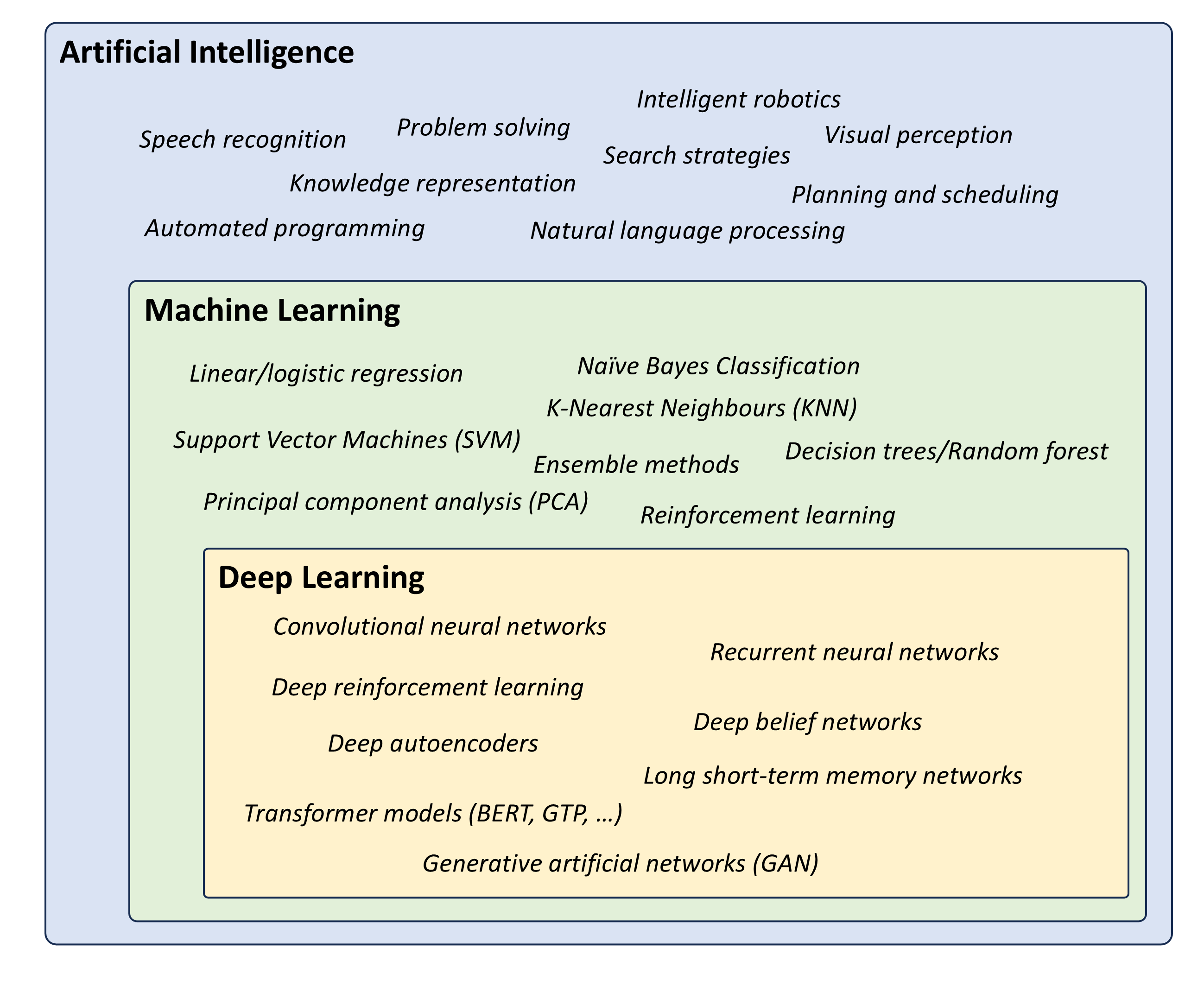
Artificial Intelligence (AI) involves techniques that equip computers to emulate human behavior, enabling them to learn, make decisions, recognize patterns, and solve complex problems in a manner akin to human intelligence.

Machine Learning (ML) is a subset of AI and uses advanced algorithms to detect patterns in large datasets, allowing machines to learn and adapt. ML algorithms use supervised or unsupervised learning methods.

Deep Learning (DL) is a subset of ML that uses neural networks for in-depth data processing and analytical tasks. It leverages multiple layers of artificial neural networks to extract high-level features from raw input data, simulating the way human brains perceive and understand the world.

Highlight:

• AI often refers to a general system or field of study. ML/DL to techniques/methods/algorithms
• reinforcement learning: interactive environment
• deep learning/neural networks: learn abstractions from raw data (feature engineering is more important for supervised ML)
• genAI/LLM/GPT: unstructured/semi-structured/structured output (beyond classification/regression)
• Prompt: what would the role of genAI be in the context of descriptive, predictive, prescriptive analytics? (descriptive: summarizing/narrative layer; predictive: limited, maybe generating code for predictive models; prescriptive: translating and explaining recommendations/trade-offs)

TODO: definition of machine learning (similar to https://www.youtube.com/watch?v=vcE9WGbi4QY) Also: AI vs ML vs deep learning (see https://www.youtube.com/watch?v=chfwJiXvBMA)

Generative AI (genAI) is a subset of DL models that generates content like text, images, or code based on provided input. Trained on vast datasets, these models detect patterns and create outputs without explicit instruction, using a mix of supervised and unsupervised learning.

Supervised and unsupervised learning

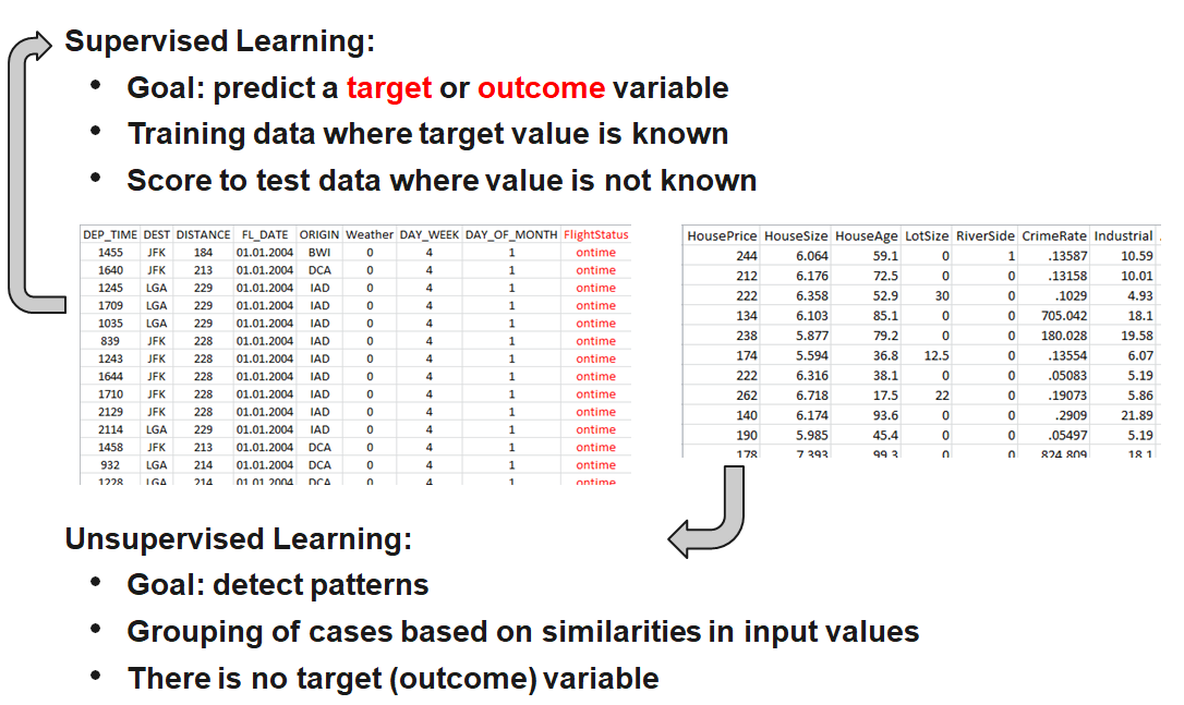
Note: Our focus will be primarily on supervised machine learning:

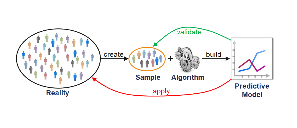
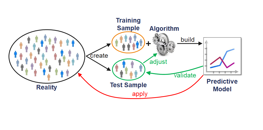
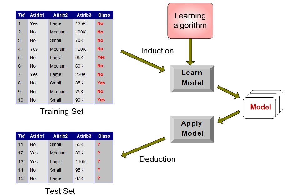
\[\underbrace{\text{Dataset}}_\text{Features, Targets} + \underbrace{\text{Learning Algorithm}}_\text{Model Class + Objective + Optimizer } \to \text{Predictive Model}\]

• Define both approaches
• Connect to what students already know:
  • “Unsupervised → clustering” (covered in exploratory data analysis)
• Emphasize: focus of this lecture + next lecture is supervised learning

The generalization problem

The traditional analytics process

Over- and underfitting

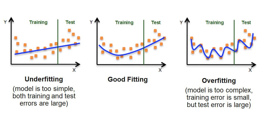
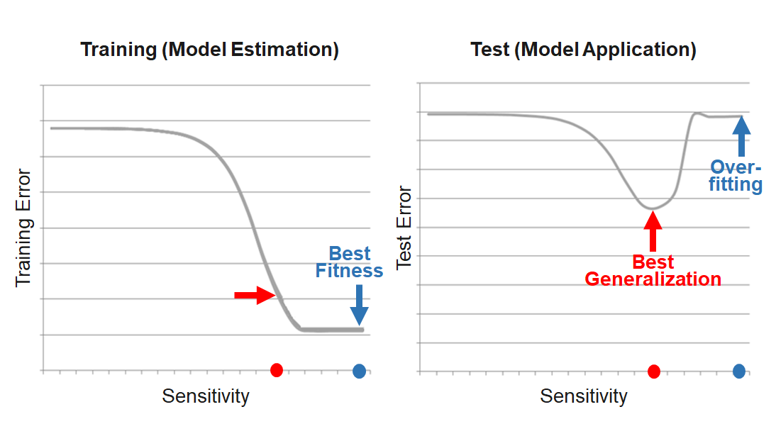
Due to the problem of overfitting, the main goal is to maximize the prediction quality and not to fit the data that is used for the model estimation as well as possible. This is equivalent to minimizing the risk that the model will have weak predictive ability.

Best fit vs. best generalization

The bias-variance tradeoff

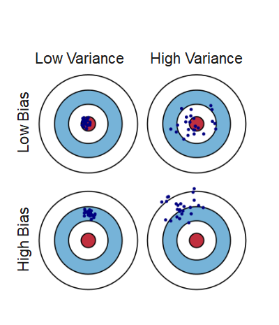
The prediction error is influenced by three components:

Error = Bias + Variance + Noise

• Bias is the inability of the used method to learn the relevant relations between the inputs and the outputs. It reflects the method quality, e.g. if a method only produces linear models.
• Variance represents the deviation resulting from the sensitivity of the created model to small fluctuations in the data.
• Typically, there is a tradeoff between bias and variance.
• Noise is everything that arises from random variations in the data. It cannot be controlled.

Generalization problem

Generalization problem: Modern machine learning models are highly flexible and trained on large datasets. While this enables them to fit complex patterns, it also creates a risk:

the model may fit the training data extremely well but fail to capture patterns that hold more generally.

The core question is therefore:

How can we tell whether a model has learned something generalizable, rather than just memorizing the data?

The machine learning workflow

The supervised machine learning workflow

Partitioning the data

Data is partitioned into training and test sets to assess whether a model generalizes beyond the data used for estimation.

• The model is trained on the training data
• Its performance is evaluated on the test data

If performance is substantially worse on the test data, the model is likely overfitting—capturing patterns specific to the training data rather than general relationships.

How can the data be split?

• Random / stratified sampling (common, but may limit reproducibility)
• Predefined lists
• Rule-based splits (e.g., first/last observations, time-based rules)

Applying training and test data

— Source: http://www.cs.kent.edu/~jin/BigData/Lecture10-ML-Classification.pptx

Problems with fixed training and test samples

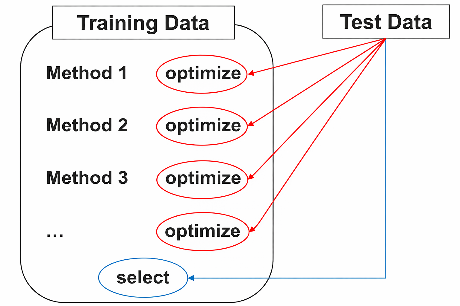
Problematic use of test data for two purposes:

1. Optimize the model training
2. Select the best model via testing the model quality

This contradicts the idea of independent testing and results in:

• Endogenization of the test data
• Selection bias

Rule: NEVER use any information from the test data for model training!

Addressing the endogeneity problem

Selection bias

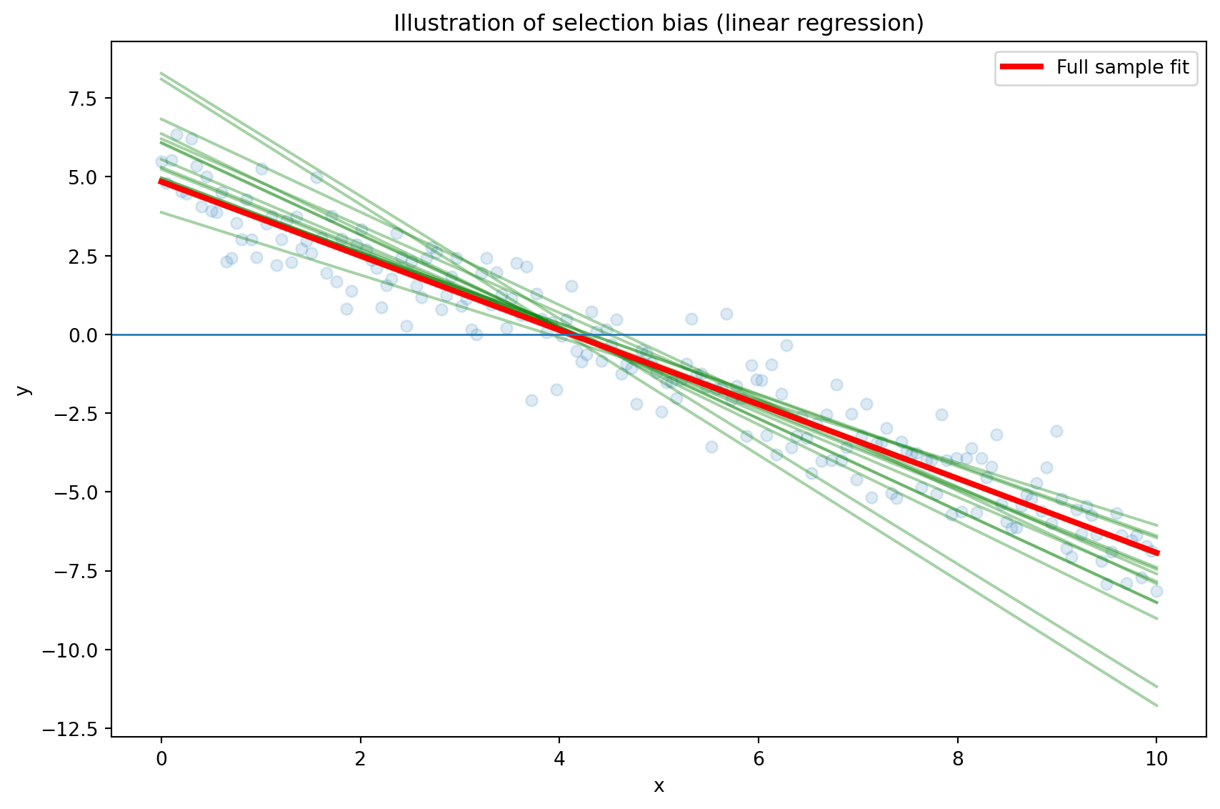
Training and test error can be highly variable, depending on precisely which observations are included in the training set and which observations are included in the validation set (selection bias).

Example of different OLS models as a result of different samples:

To avoid such problems, one can use so-called resampling methods.

Cross validation

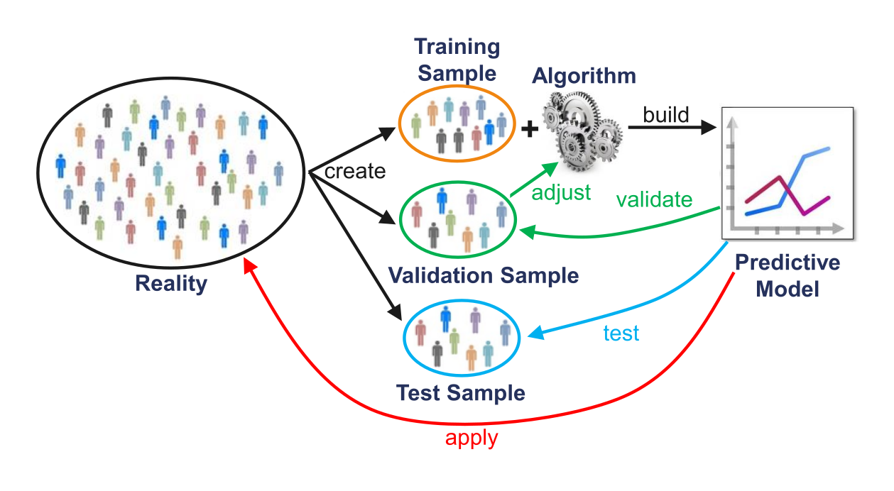
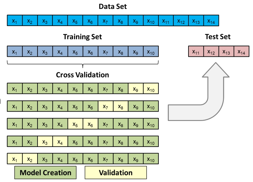
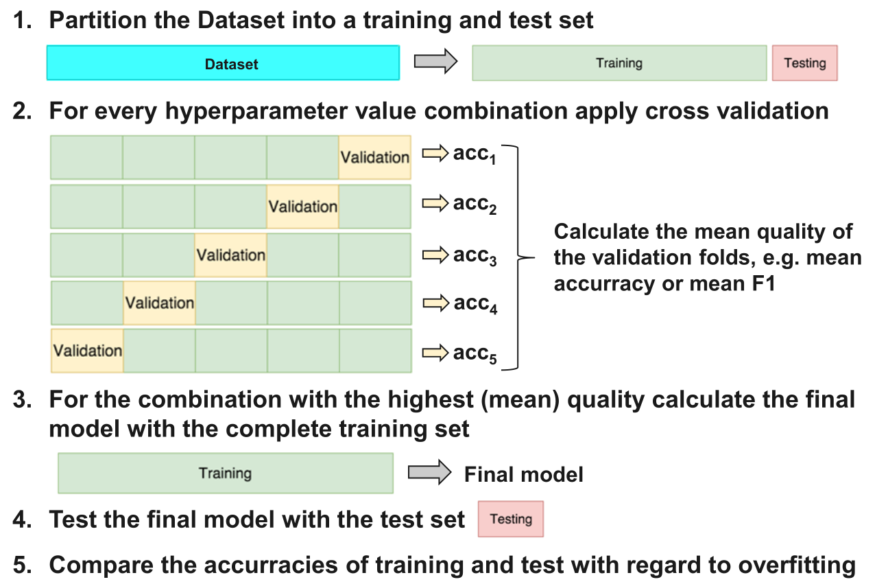
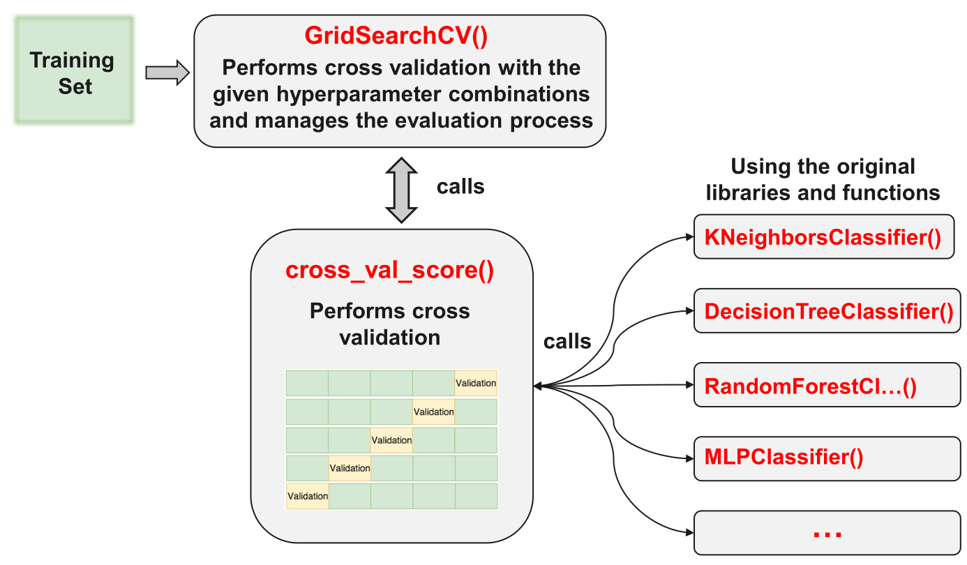
Cross validation can be used for model selection and adjustment. In these cases, cross validation is applied to the training dataset. For every iteration, k-1 folds are used for model fitting and the remaining fold for testing the model (Validation). Every time, the quality measure (e.g. accuracy) for the validation fold is captured. At the end of this step, the average and the standard deviation of the measures are calculated. The best model is the one with the best ratio in high average and low standard deviation.

Once the model type and its optimal parameters have been selected, a final model is trained using these hyper-parameters on the full training set, and the generalization quality is measured on the test set.

Cross validation and grid search

Cross validation and grid search in Python

Feature leakage

Feature leakage occurs when a model uses information that would not be available at prediction time. The model appears to perform very well on training/test data, but fails in real-world application.

Typical causes:

1. Using future information or features that are proxies of the target

Examples

• Predicting fraud
  → Feature: “transaction flagged by manual review”
• Predicting loan default
  → Feature: “number of missed payments in next 3 months”

2. Leakage from test set into training

Examples

• Scaling (mean/std) computed on the full dataset
• Feature selection using all data before splitting

Information from the test data influences the model during training Variables that are not the target itself but strongly encode it

Problem: model “sees the future” Problem: test data is no longer “unseen” Problem: model learns shortcuts instead of real patterns

Key takeaway: Only use features that are available at the time of prediction

Feature engineering

The feature engineering process

Feature engineering is the process of using domain knowledge of the data to create features that make machine learning algorithms work. When done correctly, feature engineering increases the predictive power of machine learning algorithms by creating features from raw data that help facilitate the machine learning process.

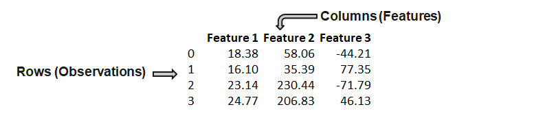
A feature (variable, attribute) is depicted by a column in a dataset. Considering a generic two-dimensional dataset, each observation is depicted by a row and each feature by a column, which will have a specific value for an observation:

Features can be of two major types.

• Raw features are obtained directly from the dataset with no extra data manipulation or engineering.
• Derived features are usually obtained from feature engineering, where we extract features from existing data attributes. A simple example would be creating a new feature “Age” from an employee dataset containing “Birthdate”.

— Source: Sarkar, D.: Understanding Feature Engineering, towardsdatascience.com and Shekhar, A.: What Is Feature Engineering for Machine Learning?, medium.com.

Variants of feature engineering

1. Transformation

• Convert features (e.g., birthdate → age)
• Build lag structures (e.g., time-lags)
• Normalization / standardization / scaling

2. Type conversion

• If numerical type is needed, transform categorical into numerical data using dummy features
• If categorical type is needed or more informative, discretize numerical features (e.g., income → poor / rich classes)

3. Feature combination

• Create interaction features (e.g., school_score = num_schools × median_school with num_schools = number of schools within 5 miles of a property and median_school = median quality score of those schools)
• Combine categories (e.g., when there are very few observations or too many dummy features)

4. Feature composition

• Build ratios (e.g., returns from prices)
• Principal Component Analysis (Dimensionality Reduction)

Scaling

Most datasets contain features that vary widely in magnitudes, units, and range.

Most machine learning algorithms have problems with this because they use distance measures or calculate gradients. The features with high magnitudes will weigh in a lot more in the distance calculations than features with low magnitudes and gradients may end up taking a long time or are not accurately calculable.

To overcome this effect, we scale the features to bring them to the same level of magnitudes. The two most discussed scaling methods are Normalization and Standardization.

Normalization (Min–Max Scaling: values in [0,1])

\[ \hat{X}_i = \frac{X_i - X_{\min}}{X_{\max} - X_{\min}} \]

Standardization (Z-score Scaling: values with mean 0 and standard deviation 1)

\[ \hat{X}_i = \frac{X_i - \mu}{\sigma} \]

For interpretation, inverse transformations are possible: \(X_i = \hat{X}_i \cdot (X_{\max} - X_{\min}) + X_{\min}\) and \(X_i = \hat{X}_i \cdot \sigma + \mu\), respectively.

Type conversion (encoding)

Many machine learning algorithms cannot work with categorical data directly. To convert categorical data to numbers, there exist two variants:

Label encoding refers to transforming the word labels into numerical form so that the algorithms can understand how to operate on them. Every categorical value is assigned to one numerical value, e.g. young → 1, middle_age → 2, old → 3. This only works in specific situations where you have somewhat continuous-like data, e.g. if the categorical feature is ordinal.

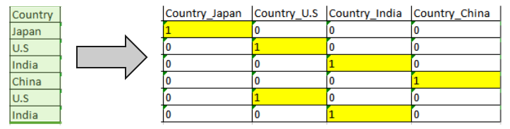
One hot encoding is a representation of a categorical variable as binary vectors. Every categorical value is assigned to an artificial binary variable. If the corresponding categorical value occurs in a data row the value of its binary replacement is equal to 1 else 0, e.g.

It is usual when creating dummy variables to have one less variable than the number of categories present to avoid perfect collinearity (dummy variable trap).

Example of feature engineering (I)

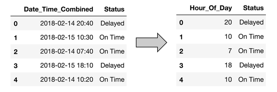
Datasets often contain date/time features. These features are rarely useful in their original form because they only contain ongoing values. However, they can be useful for extracting cyclical factors, such as weekly or seasonal effects. Suppose, we are given a data “flight date time vs status”. Then, given the date-time data, we have to predict the status of the flight.

But the status of the flight may depend on the hour of the day, not on the date-time. To analyze this, we will create the new feature “Hour_Of_Day”. Using the “Hour_Of_Day” feature, the machine will learn better as this feature is directly related to the status of the flight.

— Source: Shekhar, A.: What Is Feature Engineering for Machine Learning?, medium.com.

Example of feature engineering (II)

Suppose we are given the latitude, longitude and other data with the objective to predict the target feature “Price_Of_House”. Latitude and longitude are not of use in this context if they are alone. So, we will combine the latitude and the longitude to make one feature.

In other cases, it might be appropriate to transform latitude and longitude into categories which reflect regions, for example.

Make this Notebook Trusted to load map: File -> Trust Notebook

Example of feature engineering (III)

Suppose we are given a feature “Marital_Status” and other data with the objective to classify customers into “Creditworthy” and “Not_Creditworthy”. In the dataset the marital status has many different values, for example:

• single living alone
• single living with his parents
• married living together
• married living separately
• divorced
• divorced but living together
• registered partnerships
• living in marriage-like community
• widowed
• …

To avoid transforming into too many and maybe dominating dummy features, we can group the similar classes, e.g. in single, married, widowed.

If there exist some remaining sparse classes which cannot be assigned in a meaningful way they can be joined into a single “other” class.

Summary

• The focus is on supervised machine learning, a particular form of machine learning within AI/ML/DL, where models learn relationships between features (X) and targets (y) from labeled data. In contrast, unsupervised learning identifies structure in data without predefined labels.

• Modern machine learning models are often highly flexible and trained on large datasets, creating the risk of overfitting. The central challenge is the generalization problem: distinguishing true patterns from those specific to the training data.

• The machine learning workflow addresses this challenge by separating model development and evaluation: feature engineering, data splitting (training vs. test), model training, and performance assessment.

• Reliable model evaluation requires strict separation of training and test data, supported by techniques such as cross-validation and hyperparameter tuning, while avoiding issues like selection bias and feature leakage.

• Feature engineering is a critical step that transforms raw data into meaningful representations (e.g., scaling, encoding, feature construction), often having a stronger impact on performance than the choice of model.

Survey: Session 6

https://forms.gle/AFmpWcopjMtGfNif6

Note: Responses may be analyzed and published in anonymized form.

Please complete the survey before you leave today — thank you 🙏