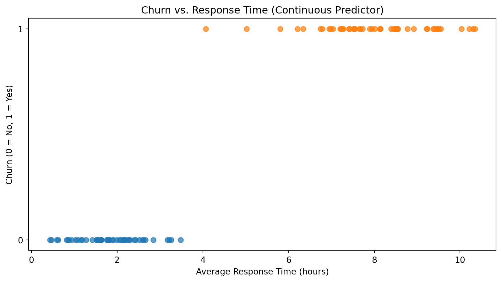
A lost customer is often a predictable customer. Firms collect many traces of customer relationships — usage, spending, support interactions, contract data. The analytical challenge is to turn these traces into an early warning system.
Typical variables in a churn dataset
Prediction goal
Predict:
\[P(\text{churn}=1 \mid X)\]
where \(X\) contains the observed customer characteristics and behaviors.

Churn prediction is a binary classification problem:
Possible approach: We could use Linear Regression with a threshold at 0.5 to classify output:
y=0y=1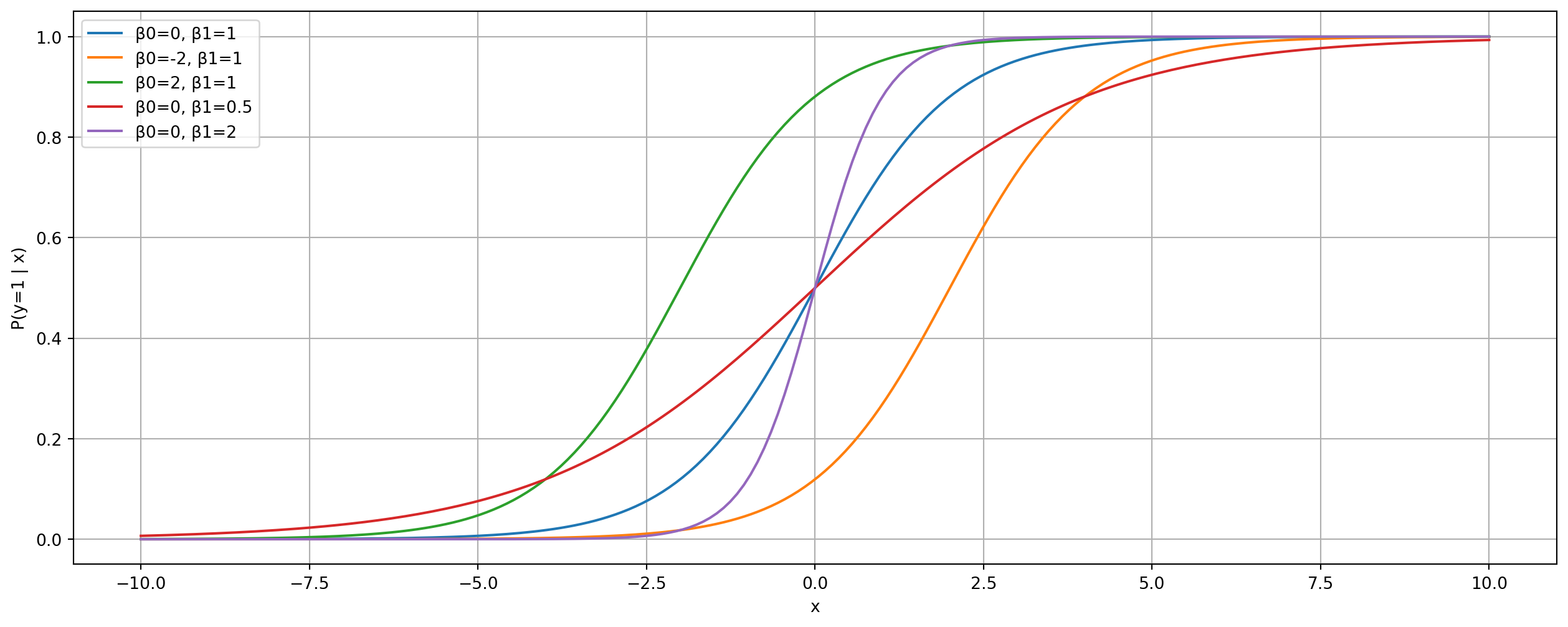
Note
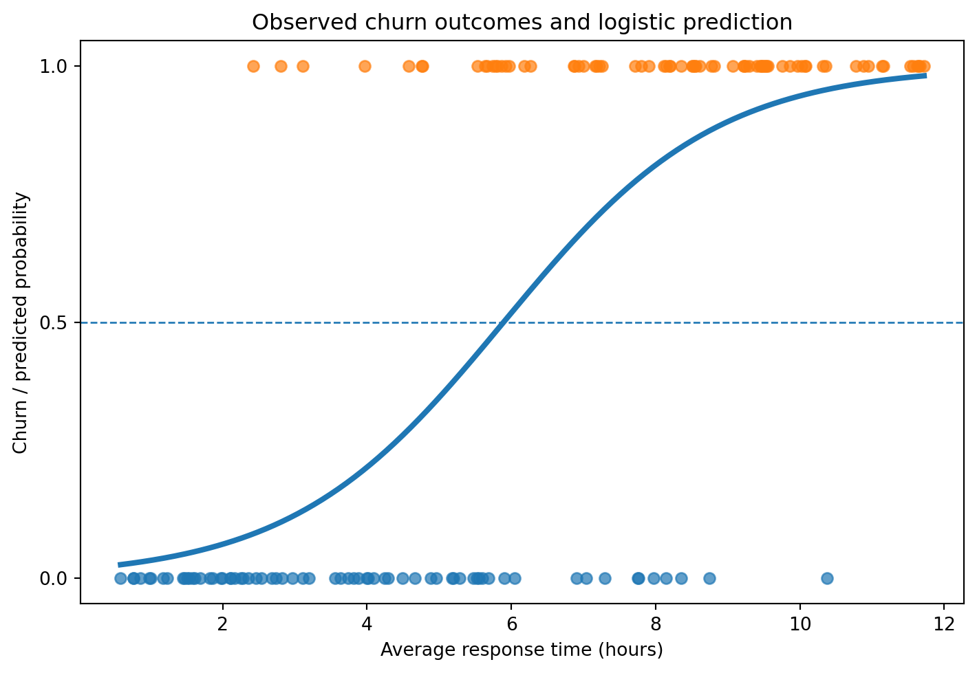
A logistic regression model predicts a probability of churn:
\[ P(\text{churn}_i=1\mid x)=\frac{1}{1+e^{-(\beta_0+\beta_1 x_i)}} \]
A threshold (such as 0.5) is needed to convert probabilities into class labels.
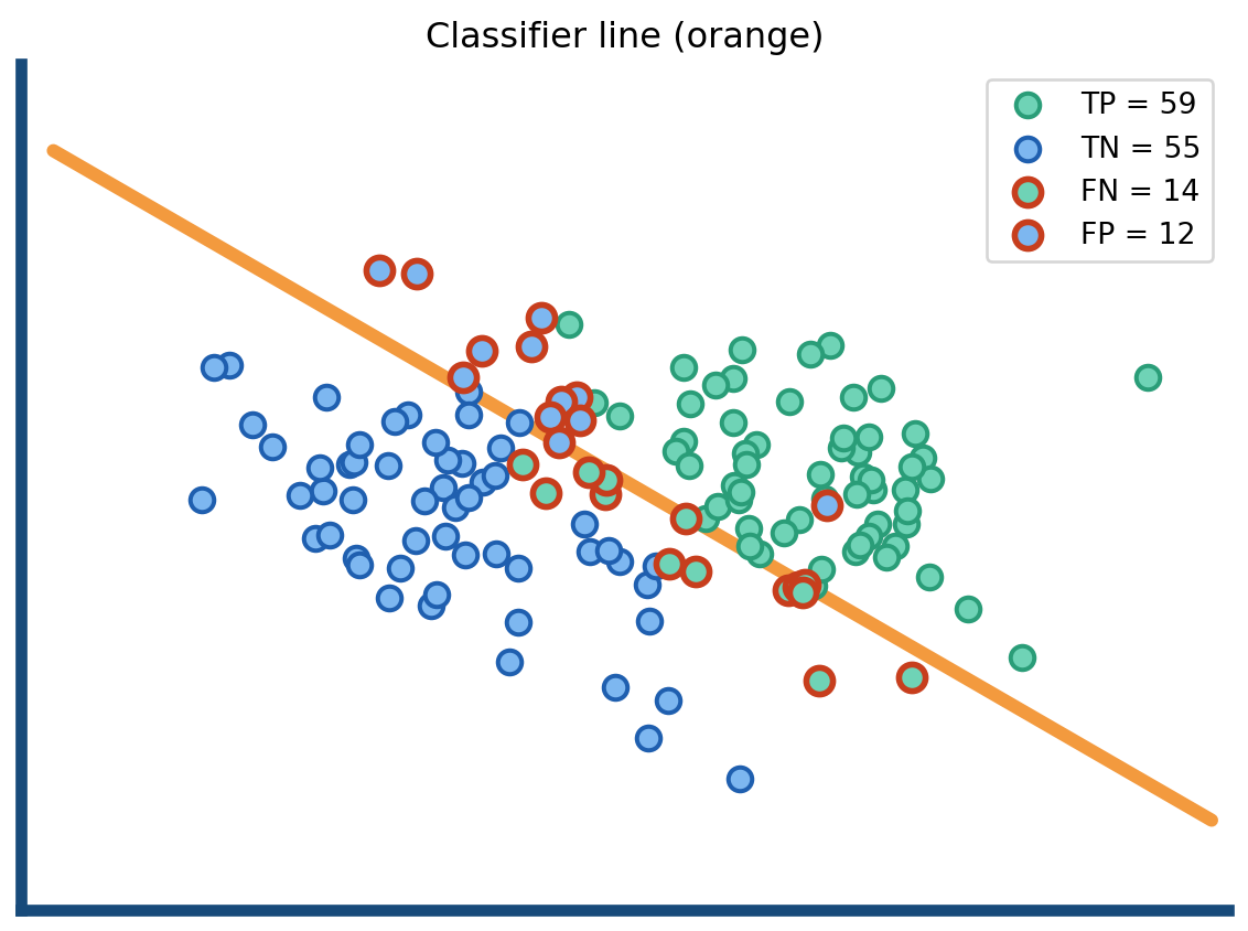
Comparing predicted vs. actual class labels allows us to evaluate the performance of a classifier like logistic regression.
Using a 0.5 threshold, predicted probabilities are turned into classes.
The confusion matrix summarizes:
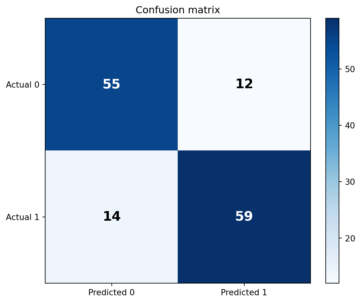
| Metric | Formula | Value | Interpretation |
|---|---|---|---|
| Accuracy | \(\frac{TP+TN}{TP+TN+FP+FN}\) | 81.4% | Overall share of correct predictions |
| Precision | \(\frac{TP}{TP+FP}\) | 83.1% | Among predicted positives, how many are actually positive? |
| Recall | \(\frac{TP}{TP+FN}\) | 80.8% | Among actual positives, how many did the model identify? |
| F1 | \(2\cdot\frac{\text{Precision}\cdot\text{Recall}}{\text{Precision}+\text{Recall}}\) | 81.9% | Balance between precision and recall |
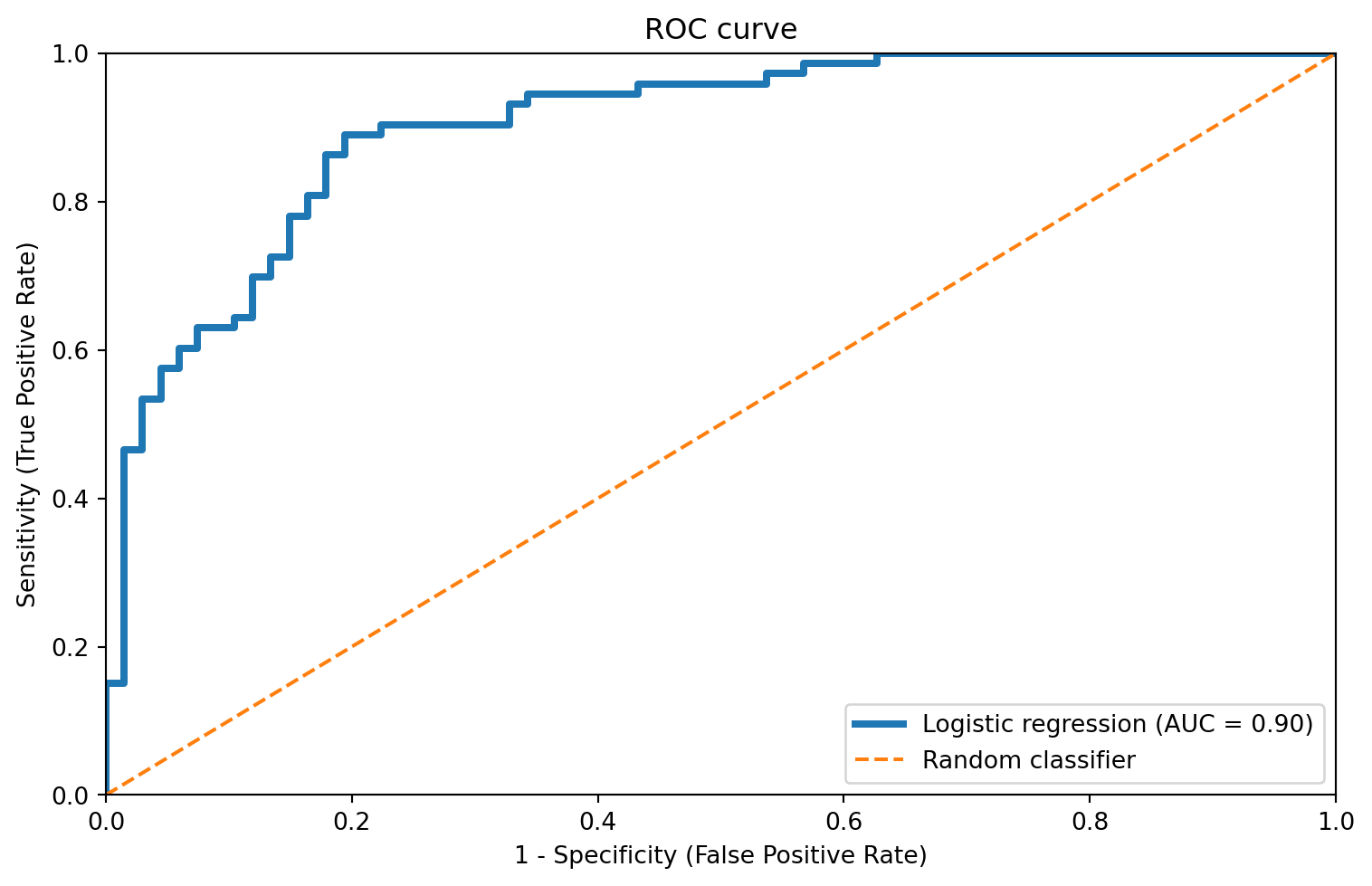
ROC (Receiver Operating Characteristic) curve summarizes the trade-off between:
As we vary the classification threshold, the model becomes more or less conservative in predicting churn = 1.
Area under the curve (AUC) summarizes ROC performance in a single number:
A good classifier achieves:
→ curves closer to the top-left corner indicate better model fit.