Exercise 5: Regression 2

import pandas as pd

df = pd.read_csv("data/credit_default.csv")
df.head()

	customer_category	income	debt_to_income	missed_payments_12m	credit_utilization	months_with_company	default
0	early_career_urban	3283.287284	0.453151	2.0	0.574281	21.0	0
1	platform_worker	1976.088070	0.597144	0.0	0.855863	39.0	1
2	platform_worker	3299.177450	0.664904	4.0	0.969859	27.0	1
3	platform_worker	2539.814969	0.505792	0.0	0.939466	7.0	0
4	early_career_urban	1655.521735	0.342233	2.0	0.461253	30.0	1

Part 1 — Analyze early-career urban borrowers with logistic regression

Task 1.1 — Prepare the subset

Create a filtered dataset that contains only customers from early-career urban borrowers.

Solution

df_ec_urban = df[df["customer_category"] == "early_career_urban"]

Task 1.2 — Estimate the model

Estimate a logistic regression model to predict credit default.

Solution

Note: You will initially encounter a ConvergenceWarning, indicating that the maximum likelihood estimation has not fully converged. To address this, increase the max_iter parameter to give the optimization algorithm sufficient iterations to converge. In practice, scaling predictors can also improve convergence and model stability.

from sklearn.linear_model import LogisticRegression

y = df_ec_urban["default"]
X = df_ec_urban.drop(columns=["default", "customer_category"])

model = LogisticRegression(max_iter=1000)
model.fit(X, y)

model.intercept_, model.coef_

(array([-0.89628046]),
 array([[-5.17141355e-04,  4.43772771e-02,  1.06127022e+00,
          1.15564749e+00, -1.62449875e-02]]))

Task 1.3 — Interpret the model

Interpret the coefficients in substantive terms:

Solution

import pandas as pd

coef_df = pd.DataFrame({"feature": X.columns, "coefficient": model.coef_[0]})

coef_df

	feature	coefficient
0	income	-0.000517
1	debt_to_income	0.044377
2	missed_payments_12m	1.061270
3	credit_utilization	1.155647
4	months_with_company	-0.016245

Note on interpretation

The coefficients shown here indicate the direction and relative strength of relationships. However, models from scikit-learn do not provide p-values or standard errors.

This means we cannot assess statistical significance directly. In applied research, p-values (e.g., from statsmodels) are typically used to evaluate whether effects are statistically reliable.

Therefore, the interpretation below focuses on magnitude and direction, not statistical significance.

Which variables increase the likelihood of default?

Solution

Variables with positive coefficients increase default risk.
In this model, the strongest positive effects are:

credit_utilization (1.16) → the strongest increase in default risk
missed_payments_12m (1.06) → substantial increase in default risk

Which variables decrease it?

Solution

Variables with negative coefficients decrease default risk.
In this model:

months_with_company (-0.02) → small decrease
income (-0.00) → very small (negligible) decrease

Which variable appears to have the strongest relationship with default?

Solution

Among the predictors, credit_utilization has the largest coefficient in absolute terms, followed closely by missed_payments_12m. This suggests that both variables are strongly associated with default risk in this model.

However, this comparison should be interpreted with caution. Because the predictors are measured on different scales (e.g., proportions, counts, income levels), the magnitude of coefficients is not directly comparable. A more rigorous comparison would require standardized variables or an analysis based on meaningful unit changes (e.g., odds ratios).

Task 1.4 — From coefficients to classification

Explain how the model moves from:

a linear combination of predictors
to a predicted probability
to a classification as default / non-default

Solution

Steps:

Linear combination (log-odds)
Logistic transformation → probability
Threshold (e.g., 0.5) → class label

# Example for one observation
z = model.intercept_[0] + (X.iloc[0] * model.coef_[0]).sum()

import numpy as np

p = 1 / (1 + np.exp(-z))

# Apply threshold
y_class = int(p >= 0.5)

p, y_class

(np.float64(0.4677867020758892), 0)

With a predicted probability of 46.8%, the observation would be classified as “no default” under a 50% threshold.

Part 2 — Probabilities and thresholds

Task 2.1 — Understanding outputs

Run the code and answer the following questions:

y_prob = model.predict_proba(X)[:, 1]
y_pred = model.predict(X)
y_prob[:5], y_pred[:5]

What is the difference between y_prob and y_pred?
Why does predict_proba return two columns?

Solution

y_prob = model.predict_proba(X)[:, 1]
y_pred = model.predict(X)
y_prob[:5], y_pred[:5]

(array([0.4677867 , 0.60611356, 0.95816943, 0.14730322, 0.7064933 ]),
 array([0, 1, 1, 0, 1]))

y_prob: probabilities for class 1 (default)
y_pred: binary predictions based on threshold (0.5 per default)

model.predict_proba(X[:5])

array([[0.5322133 , 0.4677867 ],
       [0.39388644, 0.60611356],
       [0.04183057, 0.95816943],
       [0.85269678, 0.14730322],
       [0.2935067 , 0.7064933 ]])

Column 0 → P(no default)
Column 1 → P(default)

Task 2.2 — Manual thresholding

Solution

Manually adapting the threshold t should show:

Lower threshold → more customers flagged as risky
Higher threshold → fewer customers flagged as risky

For top 20% risk:

threshold_risky = np.quantile(y_prob, 0.8)
y_pred_risky20 = (y_prob >= threshold_risky).astype(int)
threshold_risky, y_pred_risky20.sum()

(np.float64(0.6416442644835957), np.int64(39))

Flags the top 20% of customers with the highest predicted default probabilities

For safest 20%:

threshold_safe = np.quantile(y_prob, 0.2)
y_pred_safe20 = (y_prob <= threshold_safe).astype(int)
threshold_safe, y_pred_safe20.sum()

(np.float64(0.1675110069415143), np.int64(39))

Flags the bottom 20% of customers with the lowest predicted default probabilities

Low risk customers could be selected as follows:

safe_customers = df_ec_urban[y_pred_safe20 == 1]

safe_customers.head()

	customer_category	income	debt_to_income	credit_utilization	months_with_company
6	early_career_urban	2472.850226	0.165488	0.637512	20.0
22	early_career_urban	2112.056269	0.287768	0.384846	20.0
24	early_career_urban	1660.859456	0.534445	0.537737	32.0
44	early_career_urban	1793.482981	0.480555	0.335731	25.0
57	early_career_urban	2455.339943	0.543101	0.654140	25.0

Part 3 — Confusion matrix and metrics

For simplicity, model performance is evaluated on the same data used for estimation. In practice, a train/test split or cross-validation should be used.

Task 3.1 — Interpret the matrix

Solution

from sklearn.metrics import confusion_matrix

cm = confusion_matrix(y, y_pred)
cm

array([[94, 19],
       [36, 44]])

TP: 44
TN: 94
FP: 19
FN: 36

Note: the ravel() function can be helpful to access the individual values:

tn, fp, fn, tp = cm.ravel()
tn, fp, fn, tp

(np.int64(94), np.int64(19), np.int64(36), np.int64(44))

Task 3.2 — Compute key metrics

Solution (manually or based on Python)

accuracy = (tp + tn) / (tp + tn + fp + fn)
accuracy

np.float64(0.7150259067357513)

precision = tp / (tp + fp)
precision

np.float64(0.6984126984126984)

recall = tp / (tp + fn)
recall

np.float64(0.55)

Task 3.3 — Reflection

LendWise is currently trying to grow its customer base aggressively.

Discuss:

Why might the company temporarily accept a higher false-negative risk?

Solution

Growth phase:

Lower threshold → more approvals → higher growth
Accept more defaults as trade-off

Why might the same company later tighten the threshold when macroeconomic conditions worsen?

Solution

Downturn:

Higher threshold → fewer risky loans
Focus on risk control

Part 4 — ROC curve and AUC

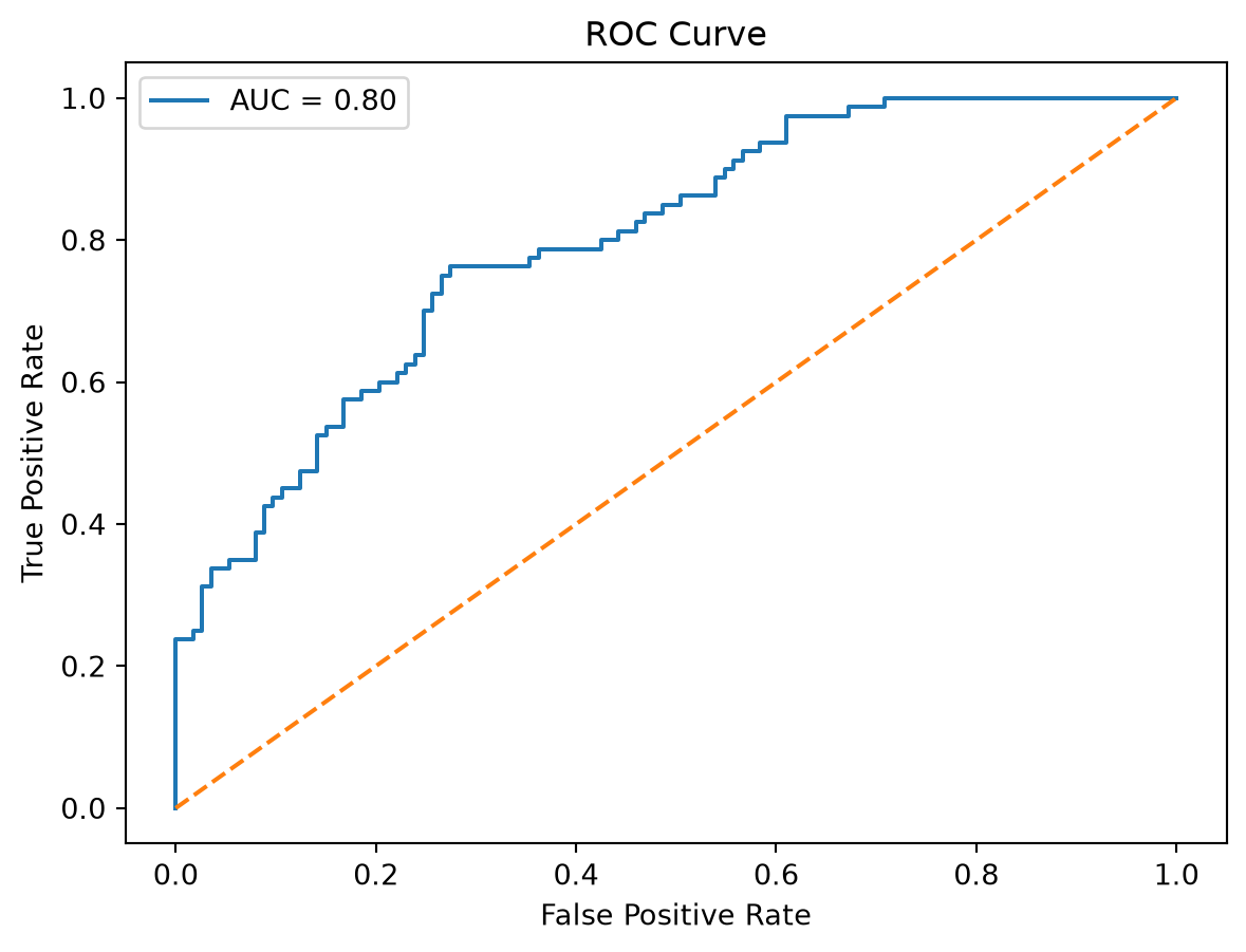
from sklearn.metrics import roc_curve, auc
import matplotlib.pyplot as plt

fpr, tpr, thresholds = roc_curve(y, y_prob)
roc_auc = auc(fpr, tpr)

# Plot ROC curve
plt.figure()
plt.plot(fpr, tpr, label=f"AUC = {roc_auc:.2f}")
plt.plot([0, 1], [0, 1], linestyle="--")  # random baseline
plt.xlabel("False Positive Rate")
plt.ylabel("True Positive Rate")
plt.title("ROC Curve")
plt.legend()
plt.show()

Task 4.1 — Understanding ROC

What does the ROC curve represent?
What are TPR and FPR?

Solution

ROC: trade-off between TPR and FPR across thresholds
TPR = TP / (TP + FN)
FPR = FP / (FP + TN)

Values for FPR, TPR at different thresholds:

roc_df = pd.DataFrame({"threshold": thresholds, "fpr": fpr, "tpr": tpr})

roc_df.head()

	threshold	fpr	tpr
0	inf	0.000000	0.0000
1	0.983469	0.000000	0.0125
2	0.813029	0.000000	0.2375
3	0.774407	0.017699	0.2375
4	0.774128	0.017699	0.2500

Task 4.2 — Interpreting AUC

What does the AUC value tell us?
What would values near 0.5, 0.7, and 1.0 suggest?

Solution

roc_auc

0.7982300884955752

0.5 → no discriminatory power (equivalent to random guessing)
~0.7 → moderate
1.0 → perfect

Task 4.3 — Threshold perspective

Why is ROC/AUC useful when the company has not yet fixed one single decision threshold?

Solution

Evaluates performance across all thresholds
Supports flexible decision-making
Enables model comparison independent of cutoff

Part 5 — Compare early-career urban borrowers and platform workers

Now repeat the same modeling steps for the segment of platform workers.

Task 5.1 — Fit the second model

Fit a logistic regression model for platform workers.

Solution

df_platform = df[df["customer_category"] == "platform_worker"]

y_platform = df_platform["default"]
X_platform = df_platform.drop(columns=["default", "customer_category"])

model_platform = LogisticRegression(max_iter=200)
model_platform.fit(X_platform, y_platform)

model_platform.intercept_, model_platform.coef_

(array([-0.8975385]),
 array([[-2.54132047e-04,  1.42011934e+00,  3.75148051e-01,
          1.38392740e+00, -1.91947960e-02]]))

Task 5.2 — Compare coefficients

Compare the coefficients across both categories.

Are the same predictors important in both groups?
Does any variable appear to matter more strongly in one group than the other?

Solution

coef_ec_urban = pd.Series(model.coef_[0], index=X.columns)
coef_platform = pd.Series(model_platform.coef_[0], index=X_platform.columns)

comparison = pd.DataFrame(
    {"Early-career urban borrowers": coef_ec_urban, "Platform workers": coef_platform}
)

comparison

	Early-career urban borrowers	Platform workers
income	-0.000517	-0.000254
debt_to_income	0.044377	1.420119
missed_payments_12m	1.061270	0.375148
credit_utilization	1.155647	1.383927
months_with_company	-0.016245	-0.019195

Some predictors matter in both groups, but their strength differs.

For both early-career urban borrowers and platform workers, credit utilization is a strong positive predictor of default, indicating that higher usage of available credit increases risk in both groups.

Income and months with company have small negative effects in both groups, suggesting slightly lower default risk with higher income and longer tenure, though these effects are minor.

Key differences emerge for debt-to-income and missed payments. For platform workers, debt-to-income is much more influential, indicating that overall debt burden plays a larger role. In contrast, for early-career urban borrowers, missed payments are more important, suggesting recent repayment behavior is a stronger signal of default risk.

Task 5.3 — Compare ROC and AUC

Compare the ROC curves and AUC values of the two models.

Which category seems easier to classify?
What might explain the difference?

Solution

y_prob_platform = model_platform.predict_proba(X_platform)[:, 1]

fpr_platform, tpr_platform, _ = roc_curve(y_platform, y_prob_platform)
roc_auc_platform = auc(fpr_platform, tpr_platform)

roc_auc, roc_auc_platform

(0.7982300884955752, 0.7167133520074697)

The model for early-career urban borrowers achieves a higher AUC (~0.80) than the model for platform workers (~0.72).

This indicates that defaults are easier to classify for early-career urban borrowers, as the model can better distinguish between defaulters and non-defaulters.

A possible explanation is that risk patterns are more clear and consistent among early-career urban borrowers (e.g., strong signals like missed payments). In contrast, platform workers may have more heterogeneous or less stable financial situations, making default harder to predict with the available variables.