Exercise 2: Data preparation and exploration

Part 1: Data structuring 1

We start with the market_data_log.csv dataset.

import pandas as pd
market_data_log_df = pd.read_csv("data/market_data_log.csv")
market_data_log_df.head()

	timestamp	logger_sys	Record
0	2024-10-16 00:00:00	FIN-PIPE-V1	SAP-DE-Tech-2023Q1-MarketCap-1154.9B
1	2023-04-25 00:00:00	FIN-PIPE-V1	SAP-DE-Tech-2023Q1-Revenue-475.6B
2	2023-01-26 00:00:00	FIN-PIPE-V1	SAP-DE-Tech-2023Q1-EBITDA-146.7B
3	2023-10-09 00:00:00	FIN-PIPE-V1	SAP-DE-Tech-2023Q2-MarketCap-1816.0B
4	2023-09-08 00:00:00	FIN-PIPE-V1	SAP-DE-Tech-2023Q2-Revenue-82.2B

Solution

1. Identify:

• Values: Examples: 2024-10-16 00:00:00, FIN-PIPE-V1, SAP, DE, 2023Q1, 1154.9
• Observations: Individual logged measurements for a specific firm and period
• Variables: Timestamp, Logger system, Firm, Country, Sector, Period, MarketCap, Revenue, EBITDA
• Units of observation: One logged firm–period record (aggregating multiple metrics)

---

2. Draft the tidy structure of the dataset (wide format):

timestamp	logger_sys	Firm	Country	Sector	Period	MarketCap	Revenue	EBITDA
2024-10-16 00:00:00	FIN-PIPE-V1	SAP	DE	Tech	2023Q1	1154.9B	475.6B	146.7B
2023-10-09 00:00:00	FIN-PIPE-V1	SAP	DE	Tech	2023Q2	1816.0B	82.2B
…	…	…	…	…	…	…	…	…

---

3. Describe how the dataset should be transformed.

• Parse encoded column:

  • The Record column contains multiple variables concatenated with -
  • Split into: Firm, Country, Sector, Period, Metric, Value

• Reshape (long → wide):

  • Pivot the Metric column into separate columns (MarketCap, Revenue, EBITDA, …)
  • Use Value as cell entries

• Optional refinement:

  • Convert Value into numeric format (e.g., remove B and cast to float)
  • Keep or drop timestamp depending on whether it represents data collection or observation time

---

4. (Optional challenge): Implement the transformation in Python (pandas)

import pandas as pd

# Load data
market_data_df = pd.read_csv("data/market_data_log.csv")

# Split encoded column
split_cols = market_data_df["Record"].str.split("-", expand=True)
split_cols.columns = ["Firm", "Country", "Sector", "Period", "Metric", "Value"]

# Combine with original dataframe
df = pd.concat([market_data_df, split_cols], axis=1)

# Pivot to wide format
df_wide = (
    df.pivot_table(
        index=["timestamp", "logger_sys", "Firm", "Country", "Sector", "Period"],
        columns="Metric",
        values="Value",
        aggfunc="first"
    )
    .reset_index()
)

df_wide.head()

Metric	timestamp	logger_sys	Firm	Country	Sector	Period	EBITDA	MarketCap	Revenue
0	2023-01-01 00:00:00	FIN-PIPE-V1	LVMH	FR	Luxury	2023Q4	26.7B	779.7B	228.0B
1	2023-01-04 00:00:00	FIN-PIPE-V1	HSBC	UK	Finance	2023Q3	190.1B	184.1B	144.1B
2	2023-01-07 00:00:00	FIN-PIPE-V1	BMW	DE	Automotive	2024Q4	99.3B	1705.8B	386.6B
3	2023-01-08 00:00:00	FIN-PIPE-V1	Total	EU	Market	2024Q3	102.0B	1004.9B	215.6B
4	2023-01-12 00:00:00	FIN-PIPE-V1	Shell	UK	Energy	2024Q2	17.6B	2272.5B	191.2B

---

Part 2: Data structuring 2

Dataset sales_data_channels_full_year.csv

import pandas as pd
sales_data_df = pd.read_csv("data/sales_data_channels_full_year.csv")
sales_data_df.head()

	Customer_ID	Region	Jan_Online	Jan_Store	Feb_Online	Feb_Store	Mar_Online	Mar_Store	Apr_Online	Apr_Store	…	Aug_Online	Aug_Store	Sep_Online	Sep_Store	Oct_Online	Oct_Store	Nov_Online	Nov_Store	Dec_Online	Dec_Store
0	ACC-E0IFD0	APAC	215	201	240	73	80	184	224	240	…	182	180	108	154	278	76	85	211	148	132
1	ACC-DPBHSA	EU	315	108	251	163	133	245	170	194	…	300	157	289	233	173	121	172	213	260	158
2	CUST-ZZPQK5	APAC	142	167	195	81	175	107	296	210	…	101	221	141	116	142	109	182	55	258	124
3	CUST-ZMF8MD	APAC	218	209	154	224	205	163	124	206	…	83	228	264	172	235	223	239	88	285	178
4	CUST-MMJBQE	EU	180	145	212	135	217	124	231	190	…	253	151	115	78	159	194	140	219	111	137

5 rows × 26 columns

Solution

1. Identify:

• Values: Numerical sales values (215, 201, 240, …)
• Observations: Individual sales measurements for a specific customer, month, and channel
• Variables: CustomerID, Region, Month, Channel, Sales
• Units of observation: A customer–month–channel combination

2. Draft the tidy structure of the dataset:

Customer_ID	Region	Month	Channel	Sales
CUST-AB12CD	EU	Jan	Online	120
CUST-AB12CD	EU	Jan	Store	95
CUST-AB12CD	EU	Feb	Online	135

3. Describe how the dataset should be transformed.

• Reshape (wide → long): Convert all monthly/channel columns into two columns
• Split the combined column (Month, Channel)

4. (Optional challenge): Implement the transformation in Python (pandas)

import pandas as pd

# Load data
sales_data_df = pd.read_csv("data/sales_data_channels_full_year.csv")

# Step 1: reshape to long format
tidy_df = sales_data_df.melt(
    id_vars=["Customer_ID", "Region"],
    var_name="Month_Channel",
    value_name="Sales"
)

# Step 2: split Month and Channel
tidy_df[["Month", "Channel"]] = tidy_df["Month_Channel"].str.split("_", expand=True)

# Step 3: drop Month_Channel
tidy_df.drop(columns=["Month_Channel"], inplace=True)

tidy_df.head()

	Customer_ID	Region	Sales	Month	Channel
0	ACC-E0IFD0	APAC	215	Jan	Online
1	ACC-DPBHSA	EU	315	Jan	Online
2	CUST-ZZPQK5	APAC	142	Jan	Online
3	CUST-ZMF8MD	APAC	218	Jan	Online
4	CUST-MMJBQE	EU	180	Jan	Online

---

Part 3: Data cleansing

Dataset messy_customer_data.csv

import pandas as pd
customers_df = pd.read_csv("data/messy_customer_data.csv")
customers_df.head()

	customer_id	date_of_birth	income	gender	signup_date	country
0	CUST_00000001809	1980-04-09	4896 USD	M	2026-12-14	USA
1	CUST_00000000695	1945-08-02	7029	F	2023-11-26	BR
2	CUST_00000000907	1971-07-25	6432	F	2024-06-25	Austria
3	CUST_00000000545	2000-03-01	6107	M	2023-06-29	JP
4	CUST_00000001848	1943-09-06	7655	F	2027-01-22	Italy
5	CUST_00000001567	1980-09-14	2244	F	2026-04-16	CH
6	CUST_00000001573	1950-04-07	3262	F	2026-04-22	India
7	CUST_00000000945	1989-08-23	3976	M	2024-08-02	BR
8	CUST_00000000819	1946-03-09	3077 USD	F	2024-03-29	NL
9	CUST_00000000830	1981-03-30	NaN	M	2024-04-09	BR
10	CUST_00000001531	1995-03-08	4667	F	2026-03-11	DE
11	CUST_00000000979	1990-01-24	NaN	F	2024-09-05	Switzerland
12	CUST_00000001576	1989-06-18	2920	F	2026-04-25	Brazil
13	CUST_00000000786	1994-06-24	6613	F	2024-02-25	IT
14	CUST_00000000071	1960-11-19	4613	F	2022-03-12	FR
15	CUST_00000001007	1989-07-09	4551	F	2024-10-03	BR
16	CUST_00000000189	1969-01-29	6779	M	2022-07-08	China
17	CUST_00000001670	1987-08-04	7295	M	2026-07-28	Munch
18	CUST_00000001270	1969-02-06	4717	F	2025-06-23	USA
19	CUST_00000001305	1989-01-13	7954	F	2025-07-28	ES

Solution

1. Identify scales of variables

• What type of scale is each variable?

  All are nominal (strings).

• What type of scale should each variable be? Assign nominal, ordinal, interval, or ratio.

  • customer_id: nominal
  • date_of_birth: interval
  • income: ratio
  • gender: nominal
  • signup_date: interval
  • country: nominal

2. Analyze data quality

Examine the dataset data/messy_customer_data.csv and run the following:

customer_df.describe()

	customer_id	date_of_birth	income	gender	signup_date	country
count	2050	1951	1948	2050	1999	2050
unique	2000	1825	1668	6	1945	33
top	CUST_00000000945	1890-01-01	200000	F	2023-13-01	AT
freq	2	10	5	995	5	93

• Summarize all data quality issues you observe.

• Missing values

  • date_of_birth
  • income
  • signup_date

• Implausible / invalid values

  • date_of_birth (e.g., 1890, future dates like 2030)
  • signup_date (e.g., invalid dates like 2023-13-01)
  • income (e.g., negative values)

• Inconsistent formats
  • income (e.g., “5000”, “5000 EUR”, “5000 USD”)
  • signup_date (multiple date formats)
• Outliers
  • income (e.g., very high values like 200000)
• Inconsistent categorical values
  • gender (M, F, Male, Female, m, f)
  • country (codes, names, typos: DE, Germany, Ger, U.S., Brasil, etc.)
• Duplicates
  • Duplicate records identifiable via repeated customer_id (high frequency)

---

3. Propose data preparation steps

• For each data quality issue, suggest how you would address it.

• Missing values: impute (e.g., median for income) or remove rows

• Implausible / invalid values: filter out or correct (e.g., negative income, invalid dates)

• Inconsistent formats: standardize (convert income to numeric, parse dates to datetime)

• Outliers: inspect and cap or remove extreme values

• Inconsistent categorical values: unify categories (e.g., gender labels, country formats)

• Duplicates: remove duplicates based on customer_id

---

4. (Optional challenge) Implement in Python (pandas)

import pandas as pd

customer_df = pd.read_csv("data/messy_customer_data.csv")

# --- Income: clean + numeric ---
customer_df["income"] = (
    customer_df["income"]
    .astype(str)
    .str.replace(r"\s*(USD|EUR)", "", regex=True)
)
customer_df["income"] = pd.to_numeric(customer_df["income"], errors="coerce")

# --- Missing values (income) ---
customer_df["income"] = customer_df["income"].fillna(customer_df["income"].median())

# --- Dates: parse ---
customer_df["date_of_birth"] = pd.to_datetime(customer_df["date_of_birth"], errors="coerce")
customer_df["signup_date"] = pd.to_datetime(customer_df["signup_date"], errors="coerce")

# --- Invalid / implausible values ---
today = pd.Timestamp.today()

# remove future DOB and very old values
customer_df = customer_df[
    (customer_df["date_of_birth"] < today) &
    (customer_df["date_of_birth"] > pd.Timestamp("1900-01-01"))
]

# remove invalid signup dates (future or NaT)
customer_df = customer_df[
    (customer_df["signup_date"] <= today)
]

# remove negative income
customer_df = customer_df[customer_df["income"] >= 0]

# --- Outliers (simple cap) ---
upper_cap = customer_df["income"].quantile(0.99)
customer_df["income"] = customer_df["income"].clip(upper=upper_cap)

# --- Gender standardization ---
customer_df["gender"] = customer_df["gender"].replace({
    "M": "Male", "m": "Male",
    "F": "Female", "f": "Female"
})

# --- Country standardization ---
country_map = {
    "Germany": "DE", "Ger": "DE", "DEU": "DE",
    "USA": "US", "U.S.": "US",
    "UK ": "UK",
    "France": "FR",
    "Spain": "ES",
    "Italy": "IT",
    "Netherlands": "NL",
    "Switzerland": "CH",
    "Austria": "AT",
    "China": "CN",
    "Japan": "JP",
    "India": "IN",
    "Brazil": "BR", "Brasil": "BR",
    "Canada": "CA",
    "Munch": "DE"
}
customer_df["country"] = customer_df["country"].replace(country_map)

# --- Remove duplicates ---
customer_df = customer_df.drop_duplicates(subset=["customer_id"])

customer_df.head()

	customer_id	date_of_birth	income	gender	signup_date	country
1	CUST_00000000695	1945-08-02	7029.0	Female	2023-11-26	BR
2	CUST_00000000907	1971-07-25	6432.0	Female	2024-06-25	AT
3	CUST_00000000545	2000-03-01	6107.0	Male	2023-06-29	JP
5	CUST_00000001567	1980-09-14	2244.0	Female	2026-04-16	CH
6	CUST_00000001573	1950-04-07	3262.0	Female	2026-04-22	IN

---

Part 4: EDA: Clustering

Now that the data is structured and cleaned, we explore whether companies group into similar patterns. Clustering helps us move from preparation to insight generation: instead of looking at firms one by one, we ask whether there are recurring profiles in the data.

Dataset: firm_data.csv

import pandas as pd
firm_data_df = pd.read_csv("data/firm_data.csv")
firm_data_df.head()

	company_id	sector	revenue	profit_margin	growth_rate	debt_ratio	market_cap	rd_intensity
0	FIRM-0095	Healthcare	2117.569743	13.382162	6.053507	0.555974	12426.889897	3.308879
1	FIRM-0015	Healthcare	457.538045	10.139487	21.504950	0.350252	5779.074618	8.710809
2	FIRM-0030	Industry	463.847307	4.131422	13.237034	0.356084	4451.965515	15.719744
3	FIRM-0158	Finance	347.980562	9.573304	16.117482	0.472141	3256.609038	31.989645
4	FIRM-0128	Tech	804.239654	0.165357	-3.346796	0.761088	1825.004761	2.082579

Solution

1. Prepare the data for clustering

We use only profit_margin and rd_intensity for clustering:

import pandas as pd

df_firm_data = pd.read_csv("data/firm_data.csv")

X = df_firm_data[["profit_margin", "rd_intensity"]]

X.head()

	profit_margin	rd_intensity
0	13.382162	3.308879
1	10.139487	8.710809
2	4.131422	15.719744
3	9.573304	31.989645
4	0.165357	2.082579

Exploratory check

X.describe()

	profit_margin	rd_intensity
count	200.000000	200.000000
mean	6.038353	11.782773
std	8.606380	10.182518
min	-18.193454	-1.006377
25%	1.165900	3.438376
50%	6.300245	7.883626
75%	11.151334	18.519914
max	26.183842	41.741721

df_firm_data[["profit_margin", "rd_intensity"]].hist(figsize=(6, 3))

array([[<Axes: title={'center': 'profit_margin'}>,
        <Axes: title={'center': 'rd_intensity'}>]], dtype=object)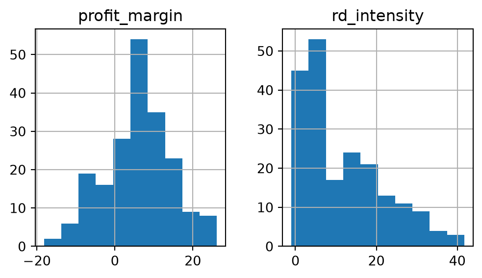

These summaries and histograms help us understand the distribution and scale of the variables.

Standardization

Since k-means is sensitive to scale differences, we standardize the variables:

from sklearn.preprocessing import StandardScaler
scaler = StandardScaler()
X_scaled = scaler.fit_transform(X)
X_scaled[:3]

array([[ 0.85543951, -0.83428853],
       [ 0.47771828, -0.30244699],
       [-0.22212786,  0.38761056]])

Scatterplot (before clustering)

import matplotlib.pyplot as plt

plt.figure(figsize=(5, 3))
plt.scatter(X_scaled[:, 0], X_scaled[:, 1], s=10)
plt.title("Standardized data (no clustering)")
plt.xlabel("profit_margin (scaled)")
plt.ylabel("rd_intensity (scaled)")
plt.show()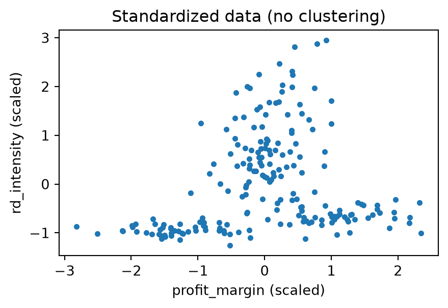

Interpretation: From the scatterplot, we might expect a small number of clusters (e.g., 3–5), depending on visible groupings.

2. Apply K-Means clustering

We try different values of k and visually inspect the cluster structure:

from sklearn.cluster import KMeans

for k in range(2, 7):
    kmeans = KMeans(n_clusters=k, random_state=42)
    labels = kmeans.fit_predict(X_scaled)

    plt.figure(figsize=(3.6, 2.8))
    plt.scatter(X_scaled[:, 0], X_scaled[:, 1], c=labels, s=10)
    plt.scatter(
        kmeans.cluster_centers_[:, 0],
        kmeans.cluster_centers_[:, 1],
        c="red", marker="x", s=60, linewidth=2
    )
    plt.title(f"k={k}", fontsize=10)
    plt.xticks([])
    plt.yticks([])
    plt.tight_layout()
    plt.show()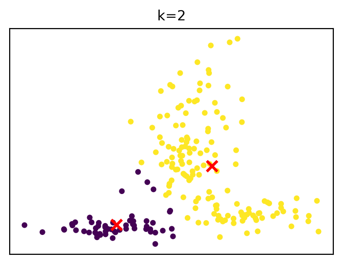

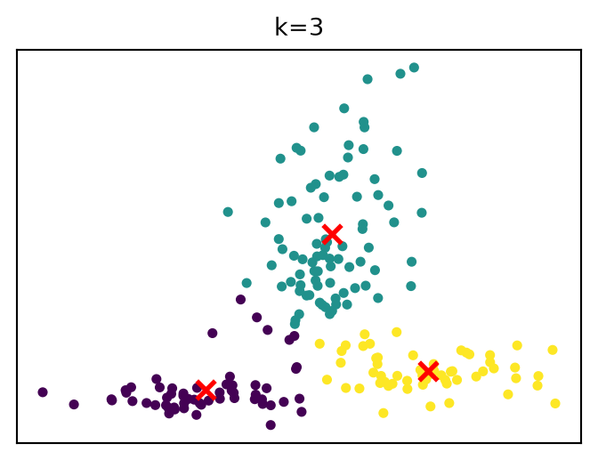
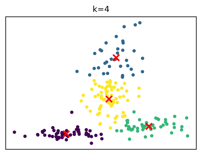
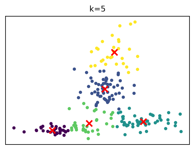
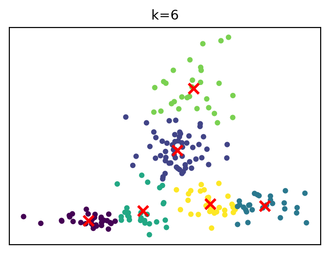
Conclusion: A value around k = 4 appears to provide a reasonable balance between simplicity and structure.

3. Add cluster labels to the dataset

We now fit the final model and store the cluster labels:

k = 4
kmeans = KMeans(n_clusters=k, random_state=42)
labels = kmeans.fit_predict(X_scaled)

df_firm_data["cluster"] = labels

df_firm_data.head()

	company_id	sector	revenue	profit_margin	growth_rate	debt_ratio	market_cap	rd_intensity	cluster
0	FIRM-0095	Healthcare	2117.569743	13.382162	6.053507	0.555974	12426.889897	3.308879	2
1	FIRM-0015	Healthcare	457.538045	10.139487	21.504950	0.350252	5779.074618	8.710809	3
2	FIRM-0030	Industry	463.847307	4.131422	13.237034	0.356084	4451.965515	15.719744	3
3	FIRM-0158	Finance	347.980562	9.573304	16.117482	0.472141	3256.609038	31.989645	1
4	FIRM-0128	Tech	804.239654	0.165357	-3.346796	0.761088	1825.004761	2.082579	0

4. Create grouped box plots

We compare revenue across clusters:

import matplotlib.pyplot as plt

df_firm_data.boxplot(column="revenue", by="cluster")
plt.title("Revenue by Cluster")
plt.suptitle("")
plt.xlabel("Cluster")
plt.ylabel("Revenue")
plt.show()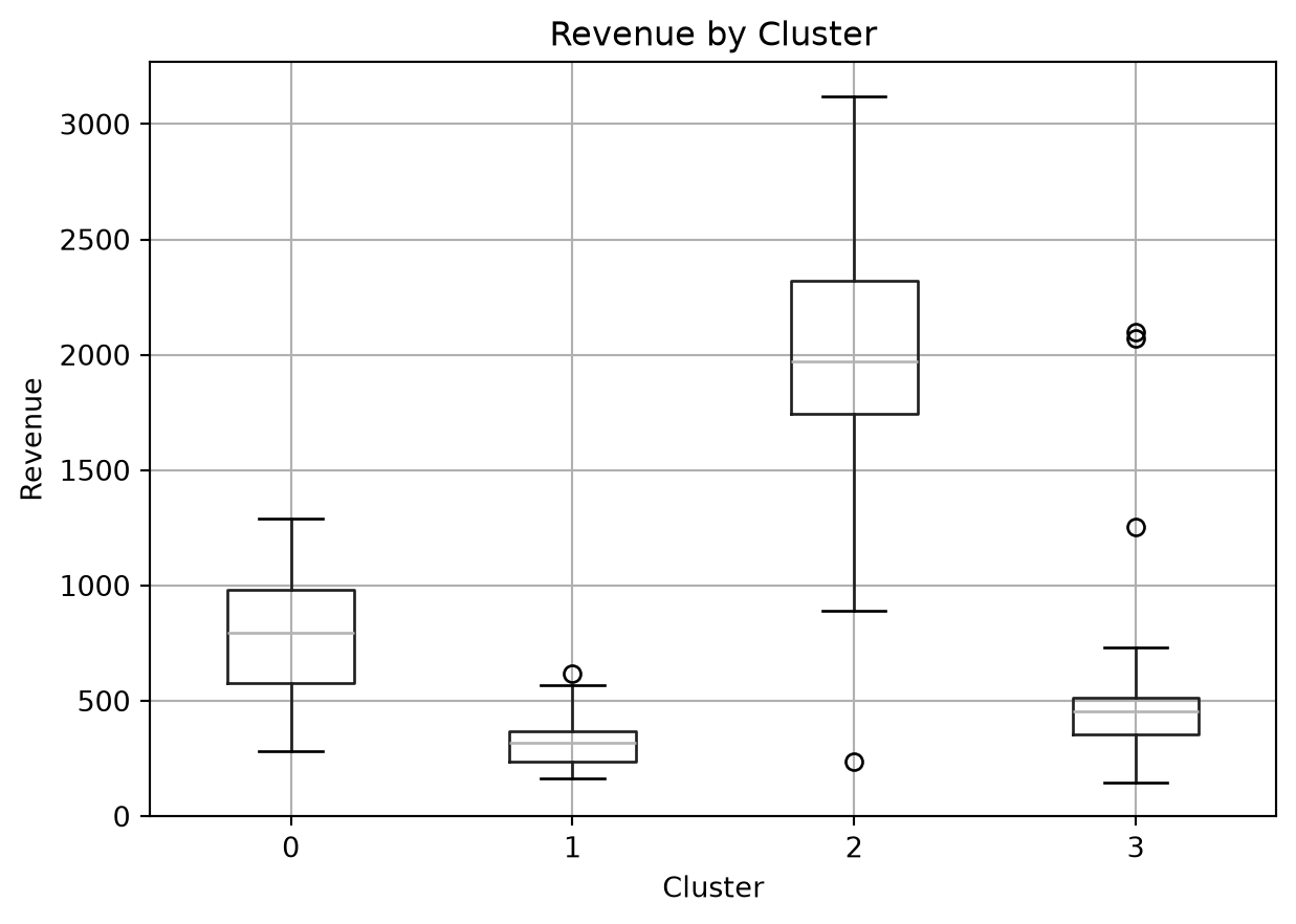

Interpretation: The box plots reveal how revenue differs across clusters, helping to characterize the identified firm profiles.